Page 177 - The Geological Interpretation of Well Logs

- LITHOLOGY RECONSTRUCTION FROM LOGS -

NEUTRON DENSITY RHOB

45 original -15] 1.95 original 2.95

NPHI

(RHOB)

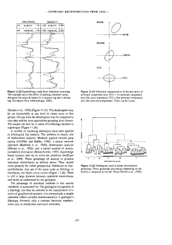
Figure 11.23 Squared logs made from statistical clustering. Figure 11.24 Schematic representation of the derivation of
The example shows the effect of plotting clustered values principal component axes. PC = Ist principal component
alongside the original values for a neutron log and a density axis (the most important), PC2 = 2nd principal component
log. (Re-drawn from Schlumberger, 1982). axis (the next most important). There can be n axes.

(Moline et ai., 1992) (Figure 11.25). The dendrogram may
be cut horizontally at any level to create more or less
groups. Groups from the dendrogram may be compared to
core data and the most appropriate grouping level chosen.
The output can now be in terms of a lithology familiar to
a geologist (Figure 11.26).
A number of clustering techniques have been applied
distance
to lithological log analysis. The problem is clearly one
of multivanate analysis. Methods applied include gene

typing (Gnffiths and Bakke, 1988), a neura] network
approach (Baldwin et ai., 1990), dendrogram analysis
(Moline et al., 1992}, and a kernel method of density
probability estimation (Mwenifumbo, 1993). Knowledge
based systems also try to solve the problems (Hoffman

et al., 1988). These groupings all attempt to produce v1 StL v
electrofacies group
statistical electrofacies as defined above. They should
more properly be called geophysical lithofacies or elec- Figure 11,25 Dendogram used to define electrofacies
groupings. These groupings can change depending on the
trolithofacies: they are of the same order as lithology or
level (i.e. distance) of cut-off. (From Moline er aé., 1992).
lithofacies, not facies sensu stricto (Figure 11.26). There
is still a large distance between statistical electrofacies
and facies as understood by the geologist.
The advantage of statistical methods is that natura]
variability is accounted for. The geological recognition of
a lithology can then be reduced to the classification of a
series of geophysical numbers: it is conceptually a simple
operation (albeit complex mathematically). A geologist’s
lithology, formerly only a concept, becomes numbers,
more easy to manipulate and more consistent.

167