Page 229 - The Geological Interpretation of Well Logs

- IMAGE LOGS -

1988). Clearly there are variations between tools and from a surface that is normal to the beam (Georgi, 1985).
loca] conditions affect the operation. With angles even slightly away from 90°, little or no
In more general terms, CBIL is indicated to have a energy will be returned to the transducer. This means that
vertical resolution of approximately 3.3 cm (0.5") hole ovality and tool tilt or non-centring will affect the
(Verdure, 1991). This figure is indicative of the resolu- sampling (Figure 13.29). The result will be dark or light
tion to expect when examining sedimentary features. stripes running up the image. Controls such as AGC
However, figures indicative from subsurface analysis are (automatic gain control) help to diminish these effects in
often much Jarger than this and an early study found that the more modem tools and they are generally (but not
features 15 cm (6") thick were not recognised (Laubach always) contained. This allows real geometric hole
et al., 1988). Experience shows that recognising especial- effects stil] to be seen, such as spiralling (Figure 13.28)
ly smaller scale sedimentary structures using the present and breakouts, especially in the time of flight plot (Figure
acoustic 100]s is difficult. 13.33).

Factors affecting acquisition
— mud weight
There are a number of factors which affect acoustic tool
Although acoustic imaging tooijs need a fluid in the bore-
acquisition in general and have an influence on quality
hoje to function, mud causes attenuation (Table 13.6).
and hence interpretation. These are briefly described
The pulse energy is absorbed and scattered by the mud
below.
particles and the beam is spread. This means that the
- borehole geometry and tool position acoustic tools will not function in heavy muds. All mud
Because the transducer pulse is highly collimated causes some loss of signai and it is suggested that quali-
(focused), it will only be reflected back to the transducer ty is poor in 8.5" holes with weights above 1.62 g/cm?’

GAMMA RAY ACOUSTIC SCANNER

0 API 100
ACOUSTIC
COMPENSATED TIME OF
CALIPERS AMPLITUDES FLIGHT
Pe eg N = $s w NON E 8 “ N

acoustic
” calipers

[gamma ray

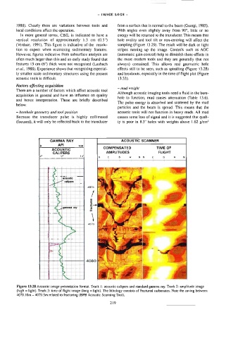
Figure 13.28 Acoustic image presentation format. Track |: acoustic calipers and standard gamma ray. Track 2: amplitde image
(high = light}. Track 3: ume of Aight image (Jong = light). The lithology consists of fractured carbonates. Note the caving between
4079.10m — 4079.5m related to fracturing (BPB Acoustic Scanning Tool).
219