Page 228 - The Geological Interpretation of Well Logs

- THE GEOLOGICAL INTERPRETATION OF WELL LOGS -

and the logging speed. In an 8.5" hole, logged at 3 m
(JOft) per minute with 250 samples per revolution and 6
travel time revolutions per second (CBIL), each sample will repre-
—<—$§$__——_ >,
sent an area of approximately 1.46 cm (.58") on the X
(
a Ss |
m Iq ar- (horizontal) axis by 0.833 cm (0.33") on the Y (vertical,
& RA depth) axis. In a 12.25” borehole the equivalent area will
S$ T amplitude be 3.04 cm (1.2") X axis by 0.833 cm (0.33") Y axis.
I
Clearly, with the too] operating from the centre of the
| I
0 20 ~100 borehole there is sample variation as hole size varies.
Production of the colour or grey scale image is the
time, microseconds .————}
major step in both amplitude and travel time image
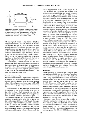
Figure 13.27 Schematic televiewer waveform pulse charac- processing. However, because of a number of unwanted
teristics. § = synchronise pulse, T = transmitted pulse, R = acquisition effects (described below), improvements are
reflected pulse (amplified). The amplitude of the returned
often made to the images themselves (of both measure-
pulse is measured and also the travel time (time of flight).
ments) by a second layer of processing. This includes
(Modified after Pasternack and Goodwill, 1983).
filtering, equalisation, edge detection and other techniques
of image processing (Wong et ai, 1989). The improve-
ments car be operator applied to workstation displays.
reflected amplitude (Figure 13.27). The time of flight is The time of flight measurements which are used to pro-
simply the time between emission, reflection off the bore- duce one of the image sets, may also be presented as an
hole wall and detection back at the transducer: it varies acoustic caliper. That is, the time of flight can be convert-
with hole geometry. The reflected amplitude is the accu- ed into a distance by accounting for the mud velocity
mulated response over a predetermined time span. That (which is monitored continuously by the tool in a special
is, the received reflected signal is converted by the sensor). This produces 250 (or other) tool] to borehole
transducer into an electrical signal, the strength of which Measurements around the full circumference of the bore-
is the reflected amplitude (simply called amplitude) hole. These values may be used to produce standard log
(Figure 13.27). The amplitude varies with the acoustic trace type caliper curves (Figure 13.28). However, they
impedance of the reflecting borehole wall, due both to may also be displayed as a polar plot that is viewed
lithology and physical features {explained below). Jooking down the hole (Figure 13.33). Some software
Acoustic imaging tools can function in a hole filled packages produce a ‘travelling polar plot’ which allows
with any fluid; water, water-based mud or oil-based mud. the operator to observe the caliper changes on the screen,
But mud attenuates the signal. In effect, the tools can only moving up the hole rather as the 100] does. There are also
be used in holes with lower density muds. CBIL uses a more complex 3D formats for screen use.
lower frequency signa] which improves operating ranges,
so that it can be used with mud densities upto 1.7-1.9 Resolution
g/cm? (15-16 lbs/gal) (Table 13.6). Feature resolution is controlled by transducer beam
characteristics, which in turn are a function of transducer
Acoustic image processing size and tool electronics (see The tools above) (Georgi,
Raw acoustic travel ime and amplitude data are general- 1985). Using experimental models, under ideal condi-
ly processed to a colour image presentation. Flight time tions the Western Atlas CBIL acoustic toot is indicated to
data can also be displayed as a continuous acoustic detect a fracture aperture with a width of 0.025 mm
caliper, either as logs or, more interestingly, in 2D or 3D (0.001") (Lincecum, 1993), much smaller than the
plan view. The image type presentations will] be discussed resolution of the transducer, Resolution is equal to the
first. radius of the pulse beam (or the transducer size in un-
The dense matrix of both amplitude and travel time focused beams). In this context, detection is the ability to
data acquired by the acoustic imaging tools, covering recognise a single object while resolution is the ability to
the entire borehole wall, is processed into colour (or separate two objects. The experiments show clearly that
grey scale) images and presented in the unwrapped bore- the acoustic tools can detect features (fractures essential-
hole log format described previously (Figure 13.2) ly) below their resolution, but that all features up to the
(Pasternack and Goodwill, 1983). The two measurements resolution resemble each other.
are plotted as two image log strips, side by side, so that Laboratory based figures are somewhat modified in
they can be compared (Figure 13.28). To make the image, subsurface practice. For example, an in-house tool used
each sample is represented by one pixel. The pixel matrix by She]l (Dudley, 1993) was able to detect in the subsur-
is built up from the 250 (or other) horizontal samples face, fractures 1 mm (0.04") or greater in width and to
from around the borehole circumference and the very resolve fractures 8 mm (0.3") apart. Other studies have
small regular depth sampling. The actual area of borehole found that the BHTY could detect fractures only with
wall represented by a pixel will depend on borehole size apertures greater than 0.5 mm (0.02") (Laubach e¢ ai,
218