Page 192 - The Handbook for Quality Management a Complete Guide to Operational Excellence

178 P r o c e s s C o n t r o l Q u a n t i f y i n g P r o c e s s Va r i a t i o n 179

per shipment. However, when part-time help is available, samples of two
crates are taken.
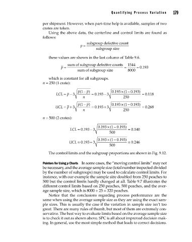
Using the above data, the centerline and control limits are found as
follows:
subgroup defective count
p =
subgroup size

these values are shown in the last column of Table 9.6.

sum of subgroup defective counts 1544
p = = = 0 193.
b
sum of subgroup size 8000
which is constant for all subgroups.
n = 250 (1 crate):

p − p) 0 193 × 1 0 193)
1
−
(
.
(
.
LCL = p − 3 = 0 193 3 = 0.1118
−
.
n 250
p( 1 p) 0 193 × ( 1 0 193)
−
− .
.
0 193 3
UCL = p + 3 = . + = 0 268
.
0
n 250
n = 500 (2 crates):
−
(
.
0 193 × 1 0 193)
.
.
−
LCL = 0 193 3 = 0 140
.
500
−
.
0 193 × ( 1 0 193)
.
UCL = 0 193 3+ = 0 246
.
.
3
500
The control limits and the subgroup proportions are shown in Fig. 9.12.
Pointers for Using p Charts In some cases, the “moving control limits” may not
be necessary, and the average sample size (total number inspected divided
by the number of subgroups) may be used to calculate control limits. For
instance, with our example the sample size doubled from 250 peaches to
500 but the control limits hardly changed at all. Table 9.7 illustrates the
different control limits based on 250 peaches, 500 peaches, and the aver-
age sample size, which is 8000 ÷ 25 = 320 peaches.
Notice that the conclusions regarding process performance are the
same when using the average sample size as they are using the exact sam-
ple sizes. This is usually the case if the variation in sample size isn’t too
great. There are many rules of thumb, but most of them are extremely con-
servative. The best way to evaluate limits based on the average sample size
is to check it out as shown above. SPC is all about improved decision mak-
ing. In general, use the most simple method that leads to correct decisions.
09_Pyzdek_Ch09_p151-208.indd 179 11/21/12 1:42 AM