Page 223 - The Mechatronics Handbook

0066_Frame_C11 Page 29 Wednesday, January 9, 2002 4:14 PM

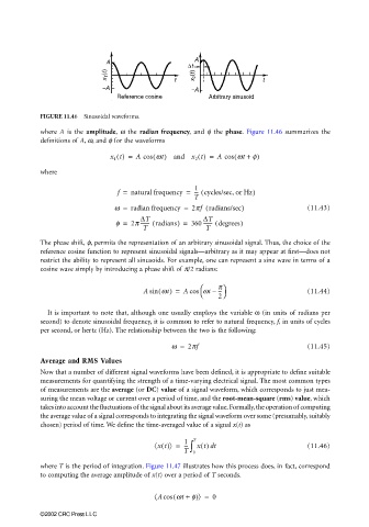
FIGURE 11.46 Sinusoidal waveforms.
where A is the amplitude, ω the radian frequency, and φ the phase. Figure 11.46 summarizes the
definitions of A, ω, and φ for the waveforms
x 1 t() = A cos wt) and x 2 t() = A cos wt + f)
(
(
where

1
f = natural frequency = --- cycles/sec, or Hz( )
T
w = radian frequency = 2pf radians/sec) (11.43)
(
∆T
∆T
f = 2p ------- radians) = 360 ------- degrees)
(
(
T T
The phase shift, φ, permits the representation of an arbitrary sinusoidal signal. Thus, the choice of the
reference cosine function to represent sinusoidal signals—arbitrary as it may appear at first—does not
restrict the ability to represent all sinusoids. For example, one can represent a sine wave in terms of a
cosine wave simply by introducing a phase shift of π/2 radians:


A sin wt) = A cos wt – p  (11.44)
(
---
2 

It is important to note that, although one usually employs the variable ω (in units of radians per
second) to denote sinusoidal frequency, it is common to refer to natural frequency, f, in units of cycles
per second, or hertz (Hz). The relationship between the two is the following:
w = 2pf (11.45)
Average and RMS Values
Now that a number of different signal waveforms have been defined, it is appropriate to define suitable
measurements for quantifying the strength of a time-varying electrical signal. The most common types
of measurements are the average (or DC) value of a signal waveform, which corresponds to just mea-
suring the mean voltage or current over a period of time, and the root-mean-square (rms) value, which
takes into account the fluctuations of the signal about its average value. Formally, the operation of computing
the average value of a signal corresponds to integrating the signal waveform over some (presumably, suitably
chosen) period of time. We define the time-averaged value of a signal x(t) as

1
〈 xt()〉 = --- ∫ T xt() t (11.46)
d
T 0
where T is the period of integration. Figure 11.47 illustrates how this process does, in fact, correspond
to computing the average amplitude of x(t) over a period of T seconds.

〈 Acos ( wt + f)〉 = 0

©2002 CRC Press LLC