Page 224 - The Mechatronics Handbook

0066_Frame_C11 Page 30 Wednesday, January 9, 2002 4:14 PM

FIGURE 11.47 Averaging a signal waveform.

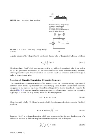
FIGURE 11.48 Circuit containing energy-storage
element.

A useful measure of the voltage of an AC waveform is the rms value of the signal, x(t), defined as follows:

1 T 2
d
--- ∫ x t() t (11.47)
x rms
T 0
Note immediately that if x(t) is a voltage, the resulting x rms will also have units of volts. If you analyze
Eq. (11.47), you can see that, in effect, the rms value consists of the square root of the average (or mean)
of the square of the signal. Thus, the notation rms indicates exactly the operations performed on x(t) in
order to obtain its rms value.

Solution of Circuits Containing Dynamic Elements
The major difference between the analysis of the resistive circuits and circuits containing capacitors and
inductors is now that the equations that result from applying Kirchhoff’s laws are differential equations,
as opposed to the algebraic equations obtained in solving resistive circuits. Consider, for example, the
circuit of Fig. 11.48 which consists of the series connection of a voltage source, a resistor, and a capacitor.
Applying KVL around the loop, we may obtain the following equation:

v S t() = v R t() + v C t() (11.48)

Observing that i R = i C , Eq. (11.48) may be combined with the defining equation for the capacitor (Eq. 4.6.6)
to obtain

1
v S t() = Ri C t() + --- ∫ t i C dt (11.49)
C – ∞

Equation (11.49) is an integral equation, which may be converted to the more familiar form of a
differential equation by differentiating both sides of the equation, and recalling that

d  t 
---- ∫ i C dt = i C t() (11.50)
dt  – ∞ 

©2002 CRC Press LLC