Page 351 - Characterization and Properties of Petroleum Fractions - M.R. Riazi

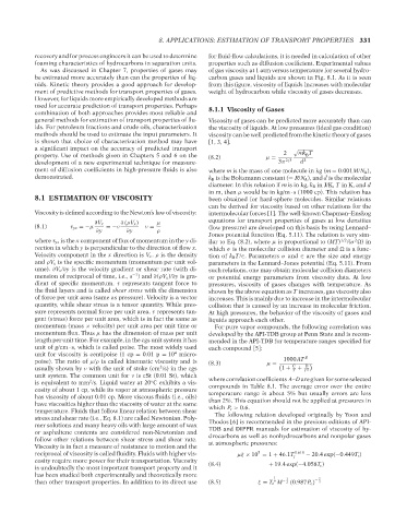
P1: JDW
AT029-Manual
June 22, 2007
AT029-Manual-v7.cls
AT029-08
14:25
8. APPLICATIONS: ESTIMATION OF TRANSPORT PROPERTIES 331
recovery and for process engineers it can be used to determine
properties such as diffusion coefficient. Experimental values
foaming characteristics of hydrocarbons in separation units. for fluid-flow calculations, it is needed in calculation of other
As was discussed in Chapter 7, properties of gases may of gas viscosity at 1 atm versus temperature for several hydro-
be estimated more accurately than can the properties of liq- carbon gases and liquids are shown in Fig. 8.1. As it is seen
uids. Kinetic theory provides a good approach for develop- from this figure, viscosity of liquids increases with molecular
ment of predictive methods for transport properties of gases. weight of hydrocarbon while viscosity of gases decreases.
However, for liquids more empirically developed methods are
used for accurate prediction of transport properties. Perhaps 8.1.1 Viscosity of Gases
combination of both approaches provides most reliable and
general methods for estimation of transport properties of flu- Viscosity of gases can be predicted more accurately than can
ids. For petroleum fractions and crude oils, characterization the viscosity of liquids. At low pressures (ideal gas condition)
methods should be used to estimate the input parameters. It viscosity can be well predicted from the kinetic theory of gases
is shown that choice of characterization method may have [1, 3, 4].
a significant impact on the accuracy of predicted transport
property. Use of methods given in Chapters 5 and 6 on the (8.2) μ = 2 mk T
B
development of a new experimental technique for measure- 3π 2/3 d 2
ment of diffusion coefficients in high-pressure fluids is also where m is the mass of one molecule in kg (m = 0.001M/N A ),
demonstrated. k B is the Boltzmann constant (= R/N A ), and d is the molecular
diameter. In this relation if mis in kg, k B in J/K, T in K, and d
in m, then μ would be in kg/m · s (1000 cp). This relation has
8.1 ESTIMATION OF VISCOSITY been obtained for hard-sphere molecules. Similar relations
can be derived for viscosity based on other relations for the
Viscosity is defined according to the Newton’s law of viscosity: intermolecular forces [1]. The well-known Chapman–Enskog
∂V x ∂ (ρV x) μ equations for transport properties of gases at low densities
(8.1) τ yx =−μ =−ν ν = (low pressure) are developed on this basis by using Lennard–
∂y ∂y ρ
Jones potential function (Eq. 5.11). The relation is very sim-
where τ yx is the x component of flux of momentum in the y di- ilar to Eq. (8.2), where μ is proportional to (MT) 1/2 /(σ )in
2
rection in which y is perpendicular to the direction of flow x. which σ is the molecular collision diameter and is a func-
Velocity component in the x direction is V x . ρ is the density tion of k B T/∈. Parameters σ and ∈ are the size and energy
and ρV x is the specific momentum (momentum per unit vol- parameters in the Lennard–Jones potential (Eq. 5.11). From
ume). ∂V x /∂y is the velocity gradient or shear rate (with di- such relations, one may obtain molecular collision diameters
−1
mension of reciprocal of time, i.e., s ) and ∂(ρV x )/∂y is gra- or potential energy parameters from viscosity data. At low
dient of specific momentum. τ represents tangent force to pressures, viscosity of gases changes with temperature. As
the fluid layers and is called shear stress with the dimension shown by the above equation as T increases, gas viscosity also
of force per unit area (same as pressure). Velocity is a vector increases. This is mainly due to increase in the intermolecular
quantity, while shear stress is a tensor quantity. While pres- collision that is caused by an increase in molecular friction.
sure represents normal force per unit area, τ represents tan- At high pressures, the behavior of the viscosity of gases and
gent (stress) force per unit area, which is in fact the same as liquids approach each other.
momentum (mass × velocity) per unit area per unit time or For pure vapor compounds, the following correlation was
momentum flux. Thus μ has the dimension of mass per unit developed by the API-TDB group at Penn State and is recom-
length per unit time. For example, in the cgs unit system it has mended in the API-TDB for temperature ranges specified for
unit of g/cm · s, which is called poise. The most widely used each compound [5]:
4
unit for viscosity is centipoise (1 cp = 0.01 p = 10 micro- B
poise). The ratio of μ/ρ is called kinematic viscosity and is (8.3) 1000AT
D
2
usually shown by ν with the unit of stoke (cm /s) in the cgs μ = 1 + C T + T 2
unit system. The common unit for ν is cSt (0.01 St), which where correlation coefficients A–D are given for some selected
2
is equivalent to mm /s. Liquid water at 20 C exhibits a vis- compounds in Table 8.1. The average error over the entire
◦
cosity of about 1 cp, while its vapor at atmospheric pressure temperature range is about 5% but usually errors are less
has viscosity of about 0.01 cp. More viscous fluids (i.e., oils)
have viscosities higher than the viscosity of water at the same than 2%. This equation should not be applied at pressures in
temperature. Fluids that follow linear relation between shear which P r > 0.6.
stress and shear rate (i.e., Eq. 8.1) are called Newtonian. Poly- The following relation developed originally by Yoon and
mer solutions and many heavy oils with large amount of wax Thodos [6] is recommended in the previous editions of API-
or asphaltene contents are considered non-Newtonian and TDB and DIPPR manuals for estimation of viscosity of hy-
follow other relations between shear stress and shear rate. drocarbons as well as nonhydrocarbons and nonpolar gases
Viscosity is in fact a measure of resistance to motion and the at atmospheric pressures:
reciprocal of viscosity is called fluidity. Fluids with higher vis- μξ × 10 = 1 + 46.1T r 0.618 − 20.4 exp(−0.449T r )
5
cosity require more power for their transportation. Viscosity (8.4) + 19.4 exp(−4.058T r )
is undoubtedly the most important transport property and it
has been studied both experimentally and theoretically more
1 1 2
6
than other transport properties. In addition to its direct use (8.5) ξ = T c M − 2 (0.987P c) − 3

--`,```,`,``````,`,````,```,,-`-`,,`,,`,`,,`---
Copyright ASTM International
Provided by IHS Markit under license with ASTM Licensee=International Dealers Demo/2222333001, User=Anggiansah, Erick
No reproduction or networking permitted without license from IHS Not for Resale, 08/26/2021 21:56:35 MDT