Page 222 - Applied Statistics Using SPSS, STATISTICA, MATLAB and R

5.3 Inference on Two Populations 203

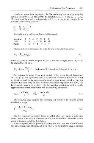
In order to assess these hypotheses, the Mann-Whitney test starts by assigning
ranks to the samples. Let the samples be denoted x 1, x 2, …, x n and y 1, y 2, …, y m.
The ranking of the x i and y i assigns ranks in 1, 2, …, n + m. As an example, let us
consider the following situation:

x i : 12 21 15 8
y i : 9 13 19

The ranking of x i and y i would then yield the result:

Variable: X Y X Y X Y X
Data: 8 9 12 13 15 19 21
Rank: 1 2 3 4 5 6 7

The test statistic is the sum of the ranks for one of the variables, say X:

W X = ∑ n = i 1 R( x ) , 5.31
i

where R(x i) are the ranks assigned to the x i. For the example above, W X = 16.
Similarly, W Y = 12 with:

N (N + ) 1
W +W = , total sum of the ranks from 1 through N = n + m.
X
Y
2

The rationale for using W X as a test statistic is that under the null hypothesis,
P(X > Y ) = ½, one expects the ranks to be randomly distributed between the x i and
y i, therefore resulting in approximately equal average ranks in each of the two
samples. For small samples, there are tables with the exact probabilities of W X. For
large samples (say m or n above 10), the sampling distribution of W X rapidly
approaches the normal distribution with the following parameters:

n (N + ) 1 nm (N + ) 1
2
µ W X = 2 ; σ W X = 12 . 5.32

Therefore, for large samples, the following test statistic with standard normal
distribution is used:

W ± 5 − µ
0
.
*
z = X W X . 5.33
σ W X

The 0.5 continuity correction factor is added when one wants to determine
critical points in the left tail of the distribution, and subtracted to determine critical
points in the right tail of the distribution.
When compared with its parametric counterpart, the t test, the Mann-Whitney
test has a high power-efficiency, of about 95.5%, for moderate to large n. In some