Page 227 - Applied Statistics Using SPSS, STATISTICA, MATLAB and R

208 5 Non-Parametric Tests of Hypotheses

A: All variables are ordinal type, measured on a 1 to 5 scale. One must note,
however, that the numeric values of the variables cannot be taken to the letter. One
could as well use a scale of A to E or use “very poor”, “poor”, “fair”, “good” and
“very good”. Thus, the sign test is the only two-sample comparison test appropriate
here.
Running the test with STATISTICA, SPSS or MATLAB yields observed one-
tailed significances of 0.0625 and 0.5 for comparisons (a) and (b), respectively.
Thus, at a 5% significance level, we do not reject the null hypothesis of
comparable distributions for pair TW and CI nor for pair MC and MA.
Let us analyse in detail the sign test results for the TW-CI pair of variables. The
respective ranks are:

TW: 4 4 3 2 4 3 3 3
CI : 3 2 3 2 4 3 2 2
Difference: + + 0 0 0 0 + +

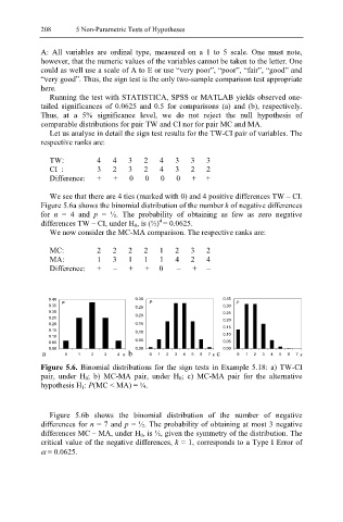
We see that there are 4 ties (marked with 0) and 4 positive differences TW – CI.
Figure 5.6a shows the binomial distribution of the number k of negative differences
for n = 4 and p = ½. The probability of obtaining as few as zero negative
4
differences TW – CI, under H 0, is (½) = 0.0625.
We now consider the MC-MA comparison. The respective ranks are:

MC: 2 2 2 2 1 2 3 2
MA: 1 3 1 1 1 4 2 4
Difference: + – + + 0 – + –

0.40 P 0.30 P 0.35 P
0.35 0.25 0.30
0.30 0.25
0.20
0.25 0.20
0.20 0.15 0.15
0.15 0.10
0.10 0.10
0.05 0.05 0.05
0.00 0.00 0.00
a 0 1 2 3 4 k b 0 1 2 3 4 5 6 7 k c 0 1 2 3 4 5 6 7 k
Figure 5.6. Binomial distributions for the sign tests in Example 5.18: a) TW-CI
pair, under H 0; b) MC-MA pair, under H 0; c) MC-MA pair for the alternative
hypothesis H 1: P(MC < MA) = ¼.

Figure 5.6b shows the binomial distribution of the number of negative
differences for n = 7 and p = ½. The probability of obtaining at most 3 negative
differences MC – MA, under H 0, is ½, given the symmetry of the distribution. The
critical value of the negative differences, k = 1, corresponds to a Type I Error of
α = 0.0625.