Page 226 - Applied Statistics Using SPSS, STATISTICA, MATLAB and R

5.3 Inference on Two Populations 207

Table 5.21b shows the results of the test; at a 5% significance level, we reject
the null hypothesis that the change of opinion was due to hazard.
In R the test is run (with the same results) as follows:

> x <- array(c(49,21,8,82),dim=c(2,2))
> mcnemar.test(x)

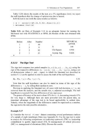
Table 5.21. (a) Data of Example 5.16 in an adequate format for running the
McNmear test with STATISTICA or SPSS, (b) Results of the test obtained with
SPSS.

Before After Number BEFORE &
1 1 49 AFTER
1 2 8 N 160
2 2 82 Chi-Square 4.966
2 1 21 Asymp. Sig. 0.026
a b

5.3.2.2 The Sign Test

The sign test compares two paired samples (x 1, y 1), (x 2, y 2), … , (x n, y n), using the
sign of the respective differences: (x 1 – y 1), (x 2 – y 2), … , (x n – y n), i.e., using a set
of dichotomous values (+ and – signs), to which the binomial test described in
section 5.1.2 can be applied in order to assess the truth of the null hypothesis:

H 0: P(x i > y i ) = P(x i < y i ) = ½ . 5.35

Note that the null hypothesis can also be stated in terms of the sign of the
differences x i – y i, by setting their median to zero.
Previous to applying the binomial test, all cases with tied decisions, x i = y i, are
removed from the analysis, and the sample size, n, adjusted accordingly. The null
hypothesis is rejected if too few differences of one sign occur.
The power-efficiency of the test is about 95% for n = 6, decreasing towards 63%
for very large n. Although there are more powerful tests for paired data, an
important advantage of the sign test is its broad applicability to ordinal data.
Namely, when the magnitude of the differences cannot be expressed as a number,
the sign test is the only possible alternative.

Example 5.17
Q: Consider the Metal Firms’ dataset containing several performance indices
of a sample of eight metallurgic firms (see Appendix E). Use the sign test in order
to analyse the following comparisons: a) leadership teamwork (TW) vs. leadership
commitment to quality improvement (CI), b) management of critical processes
(MC) vs. management of alterations (MA). Discuss the results.