Page 229 - Applied Statistics Using SPSS, STATISTICA, MATLAB and R

210 5 Non-Parametric Tests of Hypotheses

these are assigned the average of the ranks that would have been assigned without
ties. Finally, each rank gets the sign of the respective difference. For the MC and
MA variables of Example 5.17, the ranks are computed as:

MC: 2 2 2 2 1 2 3 2
MA: 1 3 1 1 1 4 2 4
MC – MA: +1 –1 +1 +1 0 –2 +1 –2

Ranks: 1 2 3 4 6 5 7
Signed Ranks: 3 –3 3 3 –6.5 3 –6.5

Note that all the magnitude 1 differences are tied; we, therefore, assign the
average of the ranks from 1 to 5, i.e., 3. Magnitude 2 differences are assigned the
average rank (6+7)/2 = 6.5.
The Wilcoxon test uses the test statistic:

+
T = sum of the ranks of the positive d i. 5.36

The rationale is that under the null hypothesis − samples are from the same
population or from populations with the same median − one expects that the sum of
the ranks for positive d i will balance the sum of the ranks for negative d i. Tables of
+
the sampling distribution of T for small samples can be found in the literature. For
large samples (say, n > 15), the sampling distribution of T + converges
asymptotically, under the null hypothesis, to a normal distribution with the
following parameters:

n ( + ) 1 n ( +n 1 )( 2 +n ) 1
n
µ = ; σ 2 = . 5.37
T + 4 T + 24

A test procedure similar to the t test can then be applied in the large sample
+
–
case. Note that instead of T the test can also use T the sum of the negative ranks.

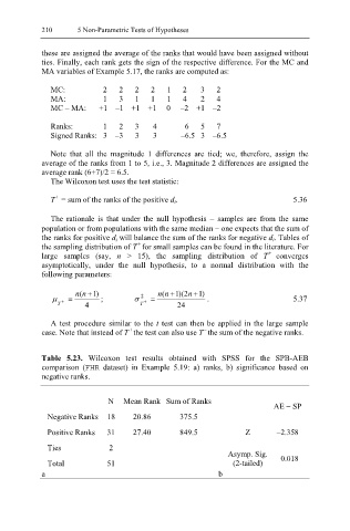
Table 5.23. Wilcoxon test results obtained with SPSS for the SPB-AEB
comparison (FHR dataset) in Example 5.19: a) ranks, b) significance based on
negative ranks.

N Mean Rank Sum of Ranks
AE − SP
Negative Ranks 18 20.86 375.5
Positive Ranks 31 27.40 849.5 Z –2.358

Ties 2
Asymp. Sig.
Total 51 (2-tailed) 0.018
a b