Page 225 - Applied Statistics Using SPSS, STATISTICA, MATLAB and R

206 5 Non-Parametric Tests of Hypotheses

H 0: After the treatment, P(+ → –) = P(– → +);
H 1: After the treatment, P(+ → –) ≠ P(– → +).

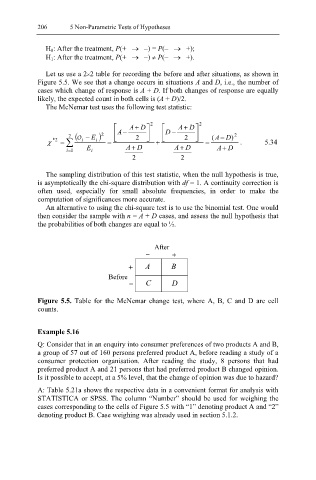
Let us use a 2×2 table for recording the before and after situations, as shown in
Figure 5.5. We see that a change occurs in situations A and D, i.e., the number of
cases which change of response is A + D. If both changes of response are equally
likely, the expected count in both cells is (A + D)/2.
The McNemar test uses the following test statistic:

 A− A+ D 2  D − A+ D  2
2 ( − E )O 2   2     2   ( A− D) 2
χ * 2 = ∑ i i = + = . 5.34
i=1 E i A+ D A+ D A+ D
2 2

The sampling distribution of this test statistic, when the null hypothesis is true,
is asymptotically the chi-square distribution with df = 1. A continuity correction is
often used, especially for small absolute frequencies, in order to make the
computation of significances more accurate.
An alternative to using the chi-square test is to use the binomial test. One would
then consider the sample with n = A + D cases, and assess the null hypothesis that
the probabilities of both changes are equal to ½.

After
+
+ A B
Before
C D

Figure 5.5. Table for the McNemar change test, where A, B, C and D are cell
counts.

Example 5.16
Q: Consider that in an enquiry into consumer preferences of two products A and B,
a group of 57 out of 160 persons preferred product A, before reading a study of a
consumer protection organisation. After reading the study, 8 persons that had
preferred product A and 21 persons that had preferred product B changed opinion.
Is it possible to accept, at a 5% level, that the change of opinion was due to hazard?
A: Table 5.21a shows the respective data in a convenient format for analysis with
STATISTICA or SPSS. The column “Number” should be used for weighing the
cases corresponding to the cells of Figure 5.5 with “1” denoting product A and “2”
denoting product B. Case weighing was already used in section 5.1.2.