Page 488 - Automotive Engineering Powertrain Chassis System and Vehicle Body

CHAP TER 1 5. 1 Modelling and assembly of the full vehicle

10000 3000
8000 2000 Ideal
Axle load (N) 6000 Front axle load Ideal rear axle brake force (N) 1000 Typical

Rear axle load
4000
2000
0 0
0 0.2 0.4 0.6 0.8 1 0 2000 4000 6000 8000 10000
Deceleration (g) Front axle brake force (N)

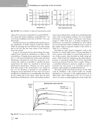
Fig. 15.1-30 Force distribution for ideal and typical braking events.
values of the convection constant hAc are around150 W K 1 and so many vehicles have a brake force distribution that
for a front disc brake installation, around 80 W K 1 for varies with vehicle loading condition. For more detailed
a rear brake installation and as low as 20 W K 1 for a rear information on brake system performance and design,
drum brake. Limpert’s 1999 work gives a detailed breakdown of
A further key factor in modelling brake performance is performance characteristics and behaviour, all of which
the distribution of brake torques around the vehicle. may be incorporated within a multibody system model of
While decelerating, the vertical loads on the axles change the vehicle using an approach similar to that shown in
due to the fact that the mass centre of the vehicle is Table 15.1-1 if desired.
above the ground. Described in some detail in Limpert’s work is the
It may be presumed that for ideal braking, the longi- function of a vehicle ABS system. The key ingredient of
tudinal forces should be distributed according to the such a system is the ability to control brake pressure in
vertical forces. Using the above expressions, the graphs in one of three modes, often described as ‘hold, dump and
Fig. 15.1-30 can be calculated for vertical axle load versus pump’. Hold is fairly self-explanatory, the wheel cylinder
deceleration. Knowing the total force necessary to de- pressure is maintained regardless of further demanded
celerate the vehicle it is possible to calculate the hori- increases in pressure from the driver’s pedal. ‘Dump’ is
zontal forces for ‘ideal’ (i.e. matched to vertical load a controlled reduction in pressure, usually at a prede-
distribution) deceleration. Plotting rear force against termined rate and ‘pump’ is a controlled increase in
front force leads to the characteristic curve shown in pressure, again usually at a predetermined rate.
Fig. 15.1-30. However, in general it is not possible to The main variable is the brake pressure p. In the 1998
arrange for such a distribution of force and so the typical work by Ozdalyan a slip control model was initially
installed force distribution is something like that shown developed as a precursor to the implementation of an
by the dashed line in the figure. Note that the ideal ABS model. This is illustrated in Fig. 15.1-31 where it
distribution of braking force varies with loading condition can be seen that on initial application of the brakes the

Braking force versus slip ratio
Braking
force
Slip angle 0
Fx(N)
OFF Camber angle 0
ON
Fz 8 kN
OFF
ON
Fz 6 kN
OFF
ON
Fz 4 kN
OFF
ON
Fz 2 kN

0.0 Slip ratio 1.0

Fig. 15.1-31 Principle of a brake slip control model.

496