Page 490 - Automotive Engineering Powertrain Chassis System and Vehicle Body

CHAP TER 1 5. 1 Modelling and assembly of the full vehicle

using the momentum available from the velocity defined only the single equation. In order to solve r 2 and r 3 this
with the initial conditions for the analysis. Ignoring rolling equation must be solved simultaneously with all the
resistance and aerodynamic drag will reduce losses but the other equations representing the motion of the vehicle.
vehicle will still lose momentum during the manoeuvre This is important particularly during cornering where the
due to the ‘drag’ components of tyre cornering forces inner and outer wheels must be able to rotate at different
generated during the manoeuvre. An example is provided speeds.
in Fig. 15.1-33 where for a vehicle lane change manoeuvre
it can be seen that during the 5 seconds taken to complete
the manoeuvre the vehicle loses about 5 km/h in the 15.1.11 Other driveline components
absence of any tractive forces at the tyres.
The emphasis with programs such as ADAMS/Car The control of vehicle speed is significantly easier than
and ADAMS/Chassis is to include a driveline model as the control of vehicle path inside a vehicle dynamics
part of the full vehicle as a means to impart torques to the model. In the real vehicle, speed is influenced by the
road wheels and hence generate tractive driving forces at engine torque, brakes and aerodynamic drag. As
the tyres. Space does not permit a detailed consideration discussed earlier these are relatively simple devices to
of driveline modelling here but as a start a simple method represent in a multibody systems model, with the ex-
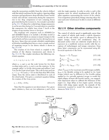
of imparting torque to the driven wheels is shown in ception of turbochargers and torque converters. Even
Fig. 15.1-34. these latter components can be represented using dif-
The rotation of the front wheels is coupled to the ferential equations of the form:
rotation of the dummy transmission part shown in
Fig. 15.1-34. The coupler introduces the following con- b
straint equation: T BOOST ¼ T 2 $T BOOST (15.1.18)
d T 1
s 1 $r 1 þ s 2 $r 2 þ s 3 $r 3 ¼ 0 (15.1.16) ðT 2 Þ¼ $ðt boost T 2 Þ (15.1.19)
dt k 2
where s 1 , s 2 and s 3 are the scale factors for the three d ðT 1 Þ¼ k 1 $ðt T 1 Þ (15.1.20)
revolute joints and r 1 , r 2 and r 3 are the rotations. In this dt boost
example suffix 1 is for the driven joint and suffixes 2 and b
3 are for the front wheel joints. The scale factors used are where T BOOST is the maximum possible torque available,
s 1 ¼ 1, s 2 ¼ 0.5 and s 3 ¼ 0.5 on the basis that 50% of the t boost is the throttle setting to be applied to the boost
torque from the driven joint is distributed to each of torque (which may be different to the throttle setting
the wheel joints. This gives a constraint equation linking applied to the normally aspirated torque to model the
the rotation of the three joints: rapid collapse of boost off-throttle) and k 1,2 are mapped,
state dependent values to calibrate the behaviour of the
(15.1.17) engine (i.e. large delays at low engine speed, reducing
r 1 ¼ 0:5r 2 þ 0:5r 3
delays with rising engine speed). An example of the
Note that this equation is not determinant. For a given statements required to model the resulting torque is
input rotation r 1 , there are two unknowns r 2 and r 3 but shown in Table 15.1-2.

REVOLUTE
TORQUE

Dummy transmission
part

COUPLER
REV

REV
Driven
wheels

Fig. 15.1-34 Simple drive torque model.

498