Page 469 - DSP Integrated Circuits

454 Chapter 10 Digital Systems

The throughput is therefore increased if the recursive calculation in the modified
FSM can be performed faster than N times the time required by the original FSM.
An FSM can be described by a state vector $ that has an element SjOi) for each
state in the FSM. The element SJ(AI) = 1 if, and only if, the FSM is in state i at time
instant n. The next state is computed by multiplying the binary state transition
matrix T(n) by the current state. For simplicity we neglect possible input signals.
We get

The scalar multiplications and additions are defined as logic AND and OR,
respectively. Iterating N steps forward we get

where

:
is the new state transition matrix. Now, since the matrix B (n+N) can be computed
outside the recursive loop, the iteration period bound has been reduced by a factor
up to N.
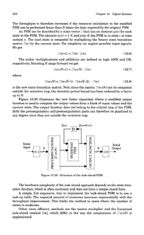
Figure 10.29 illustrates the new faster algorithm where a modified output
function is used to compute the output values from a block of input values and the
current state. The output function does not belong to the critical loop of the FSM.
Both the precomputation and postcomputation parts can therefore be pipelined to
any degree since they are outside the recursive loop.

Figure 10.29 Structure of the look-ahead FSM

The hardware complexity of the look-ahead approach depends on the state tran-
sition function, which is often nonlinear and does not have a simple closed form.
A simple, but expensive, way to implement the look-ahead FSM is to use a
look-up table. The required amount of resources increases exponentially with the
throughput improvement. This limits the method to cases where the number of
states is moderate.
Other, more efficient, methods are the matrix multiplier and the linearized
look-ahead method [14], which differ in the way the computation of D(n+N) is
implemented.