Page 667 - Engineering Digital Design

636 CHAPTER 13 / ALTERNATIVE SYNCHRONOUS FSM ARCHITECTURES

a 4-to-l MUX is indicated by the compressed EV K-maps in Fig. 13.2la. For this example,
the 8-to-l MUX will be used. Predictably, there is similarity between Eqs. (13.8) and (13.4).
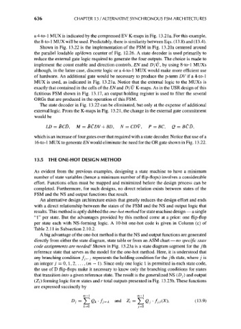
Shown in Fig. 13.22 is the implementation of the FSM in Fig. 13.20a centered around
the parallel loadable up/down counter of Fig. 12.26. A state decoder is used primarily to
reduce the external gate logic required to generate the four outputs. The choice is made to
implement the count enable and direction controls, EN and D/U, by using 8-to-l MUXs
although, in the latter case, discrete logic or a 4-to-1 MUX would make more efficient use
of hardware. An additional gate would be necessary to produce the p-term DV if a 4-to-l
MUX is used, as indicated in Fig. 13.2la. Notice that the external logic to the MUXs is
exactly that contained in the cells of the EN and D/U K-maps. As in the USR design of this
fictitious FSM shown in Fig. 13.17, an output holding register is used to filter the several
ORGs that are produced in the operation of this FSM.
The state decoder in Fig. 13.22 can be eliminated, but only at the expense of additional
external logic. From the K-maps in Fig. 13.21, the change in the external gate commitment
would be

LD = BCD, M = BCDV + BD, N = CDV, P = BC, Q = BCD,

which is an increase of four gates over that required with a state decoder. Notice that use of a
16-to-l MUX to generate EN would eliminate the need for the OR gate shown in Fig. 13.22.

13.5 THE ONE-HOT DESIGN METHOD

As evident from the previous examples, designing a state machine to have a minimum
number of state variables (hence a minimum number of flip-flops) involves a considerable
effort. Functions often must be mapped and minimized before the design process can be
completed. Furthermore, for such designs, no direct relation exists between states of the
FSM and the NS and output functions that result.
An alternative design architecture exists that greatly reduces the design effort and ends
with a direct relationship between the states of the FSM and the NS and output logic that
results. This method is aptly dubbed the one-hot method for state machine design — a single
"1" per state. But the advantages provided by this method come at a price: one flip-flop
per state each with NS-forming logic. A 10-bit one-hot code is given in Column (c) of
Table 2.11 in Subsection 2.10.2.
A big advantage of the one-hot method is that the NS and output functions are generated
directly from either the state diagram, state table or from an ASM chart — no specific state
code assignments are needed! Shown in Fig. 13.23a is a state diagram segment for the jth
reference state that serves as the model for the one-hot method. Here, it is understood that
any branching condition //<_/ represents the holding condition for the y'th state, where j is
an integer j = 0, 1, 2,... , (m — 1). Since only one logic 1 is permitted in each state code,
the use of D flip-flops make it necessary to know only the branching conditions for states
that transition into a given reference state. The result is the generalized NS (Dj) and output
(Z/) forming logic for m states and r total outputs presented in Fig. 13.23b. These functions
are expressed succinctly by
i n — 1 m — \
Dj = Qk-fj^ k and Z, = Qj-fj,,(X), (13.9)