Page 670 - Engineering Digital Design

638 CHAPTER 1 3 / ALTERNATIVE SYNCHRONOUS FSM ARCHITECTURES

D Q f + Q + Q f
o = o o^o 1 Vi 2 o<- 2
D, = Q 0 V 0 + Q, V, + Q 2f^

D f
u (rn-i} *™u
i (rn -i)<— i
m-i
mi=Qn /m n n+Qitm n 1+CU, n o+"'+ Q <t „ <
m-l (m-t)
d. (rn-l) <—c

(a) (b)
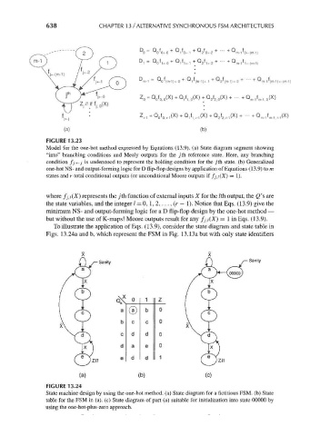
FIGURE 13.23
Model for the one-hot method expressed by Equations (13.9). (a) State diagram segment showing
"into" branching conditions and Mealy outputs for the y'th reference state. Here, any branching
condition //<-_/ is understood to represent the holding condition for the j'th state, (b) Generalized
one-hot NS- and output-forming logic for D flip-flop designs by application of Equations (13.9) to m
states and r total conditional outputs (or unconditional Moore outputs if fjj(X) = 1).

where fj,i(X ) represents the y'th function of external inputs X for the /th output, the £>'s are
the state variables, and the integer / = 0, 1, 2, . . . , (r — 1). Notice that Eqs. (13.9) give the
minimum NS- and output-forming logic for a D flip-flop design by the one-hot method —
but without the use of K-maps! Moore outputs result for any fj,i(X ) = 1 in Eqs. (13.9).
To illustrate the application of Eqs. (13.9), consider the state diagram and state table in
Figs. 13.24a and b, which represent the FSM in Fig. 13.13a but with only state identifiers

Sanity

X ° 1 Z
a ® b 0
b c c 0

c d d 0
d a e 0

e d d 1
IZiT
(a) (b) (c)
FIGURE 13.24
State machine design by using the one-hot method, (a) State diagram for a fictitious FSM. (b) State
table for the FSM in (a), (c) State diagram of part (a) suitable for initialization into state 00000 by
using the one-hot-plus-zero approach.