Page 42 - Finite Element Modeling and Simulations with ANSYS Workbench

Bars and Trusses 27

where

k = ∫ B ( T E B)dV (2.20)
V
is the element stiffness matrix.
Equation 2.20 is a general result which can be used for the construction of other types
of elements.
Now, we evaluate Equation 2.20 for the bar element by using Equation 2.14
L  −1/L   1 −  1
k = ∫ 1/L    −1/L 1/LAdx = EA  −1 1 

E


0   L  
which is the same as we derived earlier using the direct method.
Note that from Equations 2.16 and 2.20, the strain energy in the element can be written as
1
T
U = uku (2.21)
2
In the future, once we obtain an expression like Equation 2.16, we can immediately rec-
ognize that the matrix in between the displacement vectors is the stiffness matrix. Recall
that for a spring, the strain energy can be written as
1 1
U = k∆ 2 = ∆ T k∆
2 2
Thus, result (2.21) goes back to the simple spring case again.

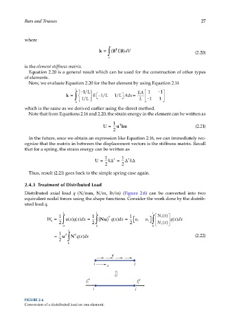
2.4.3 Treatment of Distributed Load
Distributed axial load q (N/mm, N/m, lb/in) (Figure 2.6) can be converted into two
equivalent nodal forces using the shape functions. Consider the work done by the distrib-
uted load q,

L L L
∫
1 1 T 1  Nx()
i
W q = ∫ u xqxdx = ∫ (Nu ) q xdx =   u i u j      qx dx
()
()
()
()
2 2 2  Nx() 
j
0 0 0
L
1
= 2 u T ∫ N T qx dx (2.22)
()
0
q
i x j
f i q f j q
i j

FIGURE 2.6
Conversion of a distributed load on one element.