Page 43 - Finite Element Modeling and Simulations with ANSYS Workbench

28 Finite Element Modeling and Simulation with ANSYS Workbench

q

1 2 3

qL/2 qL qL/2
1 2 3

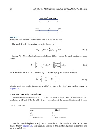
FIGURE 2.7
Conversion of a distributed load with constant intensity q on two elements.

The work done by the equivalent nodal forces are

1 1 1
q
= f u i + f u j = uf (2.23)
q
T
W f q i j q
2 2 2
Setting W q = W f q and using Equations 2.22 and 2.23, we obtain the equivalent nodal force
vector
 i f  L L  i Nx 
q
()


T
 =
()
()
f q =  q ∫ N qx dx = ∫  Nx  qx dx (2.24)
 j f    0 0  j () 
which is valid for any distributions of q. For example, if q is a constant, we have
L 1 − /  qL 2/ 
xL
f q = q ∫   dx =   (2.25)
/
/
0  xL   qL 2 
that is, equivalent nodal forces can be added to replace the distributed load as shown in
Figure 2.7.
2.4.4 Bar Element in 2-D and 3-D
To analyze the truss structures in 2-D or 3-D, we need to extend the 1-D bar element for-
mulation to 2-D or 3-D. In the following, we take a look at the formulation for the 2-D case.

2.4.4.1 2-D Case

Local Global
x, y X, Y
i , ′ uv i ′ u i , v i
1 DOF at each node 2 DOFs at each node

Note that lateral displacement ′ v i does not contribute to the stretch of the bar within the
linear theory (Figure 2.8). Displacement vectors in the local and global coordinates are
related as follows: