Page 136 - Fluid-Structure Interactions Slender Structure and Axial Flow (Volume 1)

118 SLENDER STRUCTURES AND AXIAL FLOW

3.5.3 The effect of dissipation

We next consider the effect of dissipation on stability. As first shown by Ziegler (1952)
for the nonconservative system of a double pendulum subjected to a follower load, weak
damping may actually destabilize the system. The same was found in the study of stability
of a compliant surface over which there exists a flow (Benjamin 1960, 1963). Benjamin
classified the various possible modes of instability into three distinct classes, according
to the mode of energy exchange between fluid and solid. Benjamin shows that ‘class A’
waves are destabilized by damping, and Landahl (1962) has contributed to the discussion
and clarification of this paradox; see also Section 3.5.5. It was in this same period that it
was found that cantilevered pipes conveying fluid can also be destabilized by dissipation
(Pafdoussis 1963). Subsequently, a considerable amount of work has been done on this
topic [e.g. by Gregory & Paidoussis (1966b), Nemat-Nasser et al. (1966), Bolotin &
Zhinzher (1969), PaIdoussis (1970), Paidoussis & Issid (1974)l.
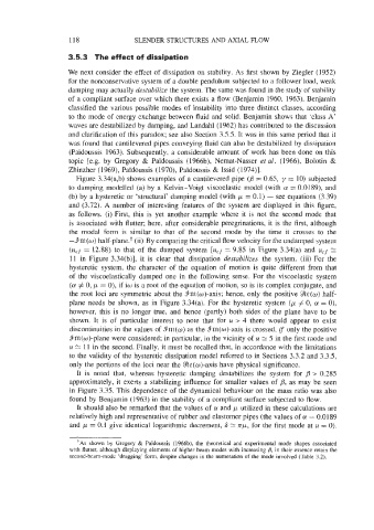
Figure 3.34(a,b) shows examples of a cantilevered pipe (’ = 0.65, y = 10) subjected
to damping modelled (a) by a Kelvin-Voigt viscoelastic model (with a = 0.0189), and
(b) by a hysteretic or ‘structural’ damping model (with p = 0.1) - see equations (3.39)
and (3.72). A number of interesting features of the system are displayed in this figure,
as follows. (i) First, this is yet another example where it is not the second mode that
is associated with flutter; here, after considerable peregrinations, it is the first, although
the modal form is similar to that of the second mode by the time it crosses to the
-9m(w) half-plane.t (ii) By comparing the critical flow velocity for the undamped system
(u,f = 12.88) to that of the damped system [u,~ = 9.85 in Figure 3.34(a) and ucf 2:
11 in Figure 3.34(b)], it is clear that dissipation destabilizes the system. (iii) For the
hysteretic system, the character of the equation of motion is quite different from that
of the viscoelastically damped one in the following sense. For the viscoelastic system
(a # 0, p = 0), if iw is a root of the equation of motion, so is its complex conjugate, and
the root loci are symmetric about the 9m(w)-axis; hence, only the positive %e(w) half-
plane needs be shown, as in Figure 3.34(a). For the hysteretic system (@ # 0, 01 = 0),
however, this is no longer true, and hence (partly) both sides of the plane have to be
shown. It is of particular interest to note that for u > 4 there would appear to exist
discontinuities in the values of 9m(w) as the 9m(o)-axis is crossed, if only the positive
9m(w)-plane were considered; in particular, in the vicinity of u 2: 5 in the first mode and
u 11 in the second. Finally, it must be recalled that, in accordance with the limitations
to the validity of the hysteretic dissipation model referred to in Sections 3.3.2 and 3.3.5,
only the portions of the loci near the %e(w)-axis have physical significance.
It is noted that, whereas hysteretic damping destabilizes the system for fi > 0.285
approximately, it exerts a stabilizing influence for smaller values of P, as may be seen
in Figure 3.35. This dependence of the dynamical behaviour on the mass ratio was also
found by Benjamin (1963) in the stability of a compliant surface subjected to flow.
It should also be remarked that the values of a and p utilized in these calculations are
relatively high and representative of rubber and elastomer pipes (the values of 01 = 0.0189
and p = 0.1 give identical logarithmic decrement, 6 2 np, for the first mode at u = 0).

‘As shown by Gregory & Pai’doussis (1966b). the theoretical and experimental mode shapes associated
with flutter, although displaying elements of higher beam modes with increasing ,fJ, in their essence retain the
second-beam-mode ‘dragging’ form, despite changes in the numeration of the mode involved (Table 3.2).