Page 100 - T. Anderson-Fracture Mechanics - Fundamentals and Applns.-CRC (2005)

1656_C02.fm Page 80 Thursday, April 14, 2005 6:28 PM

80 Fracture Mechanics: Fundamentals and Applications

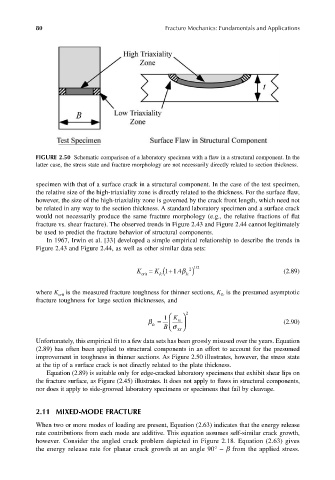
FIGURE 2.50 Schematic comparison of a laboratory specimen with a flaw in a structural component. In the
latter case, the stress state and fracture morphology are not necessarily directly related to section thickness.

specimen with that of a surface crack in a structural component. In the case of the test specimen,
the relative size of the high-triaxiality zone is directly related to the thickness. For the surface flaw,
however, the size of the high-triaxiality zone is governed by the crack front length, which need not
be related in any way to the section thickness. A standard laboratory specimen and a surface crack
would not necessarily produce the same fracture morphology (e.g., the relative fractions of flat
fracture vs. shear fracture). The observed trends in Figure 2.43 and Figure 2.44 cannot legitimately
be used to predict the fracture behavior of structural components.
In 1967, Irwin et al. [33] developed a simple empirical relationship to describe the trends in
Figure 2.43 and Figure 2.44, as well as other similar data sets:

K = K Ic( + Ic )11 4 . β 2 12 / (2.89)
crit

where K is the measured fracture toughness for thinner sections, K is the presumed asymptotic
Ic
crit
fracture toughness for large section thicknesses, and
K 
β = 1   σ   2 (2.90)
Ic
Ic
B 
YS
Unfortunately, this empirical fit to a few data sets has been grossly misused over the years. Equation
(2.89) has often been applied to structural components in an effort to account for the presumed
improvement in toughness in thinner sections. As Figure 2.50 illustrates, however, the stress state
at the tip of a surface crack is not directly related to the plate thickness.
Equation (2.89) is suitable only for edge-cracked laboratory specimens that exhibit shear lips on
the fracture surface, as Figure (2.45) illustrates. It does not apply to flaws in structural components,
nor does it apply to side-grooved laboratory specimens or specimens that fail by cleavage.

2.11 MIXED-MODE FRACTURE

When two or more modes of loading are present, Equation (2.63) indicates that the energy release
rate contributions from each mode are additive. This equation assumes self-similar crack growth,
however. Consider the angled crack problem depicted in Figure 2.18. Equation (2.63) gives
the energy release rate for planar crack growth at an angle 90° − β from the applied stress.