Page 282 - Geothermal Energy Systems Exploration, Development, and Utilization

258 5 Geothermal Reservoir Simulation
Fluid pressure Fluid heat at
Ratio of efficiency of heat extraction, CO 2 : H 2 O 5 CO 2 more efficient
10 MPa eq. 1000 m
20 MPa eq. 2000 m
10
30 MPa eq. 3000 m
40 MPa eq. 4000 m
7
4
3
2

1

Line at which efficiency of heat
extraction using CO 2 is the same
as that of water
300 350 400 450 H 2 O more efficient
Reservoir temperature
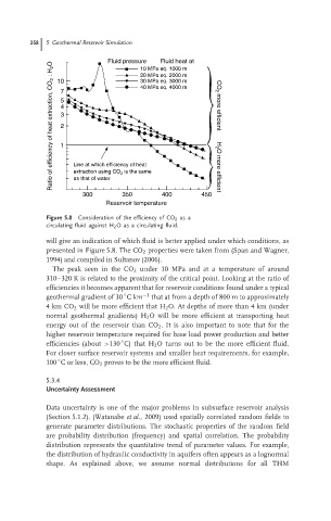
Figure 5.8 Consideration of the efficiency of CO 2 as a
circulating fluid against H 2 Oas a circulatingfluid.

will give an indication of which fluid is better applied under which conditions, as
presented in Figure 5.8. The CO 2 properties were taken from (Span and Wagner,
1994) and compiled in Sultanov (2006).
The peak seen in the CO 2 under 10 MPa and at a temperature of around
310–320 K is related to the proximity of the critical point. Looking at the ratio of
efficiencies it becomes apparent that for reservoir conditions found under a typical
◦
geothermal gradient of 30 Ckm −1 that at from a depth of 800 m to approximately
4km CO 2 will be more efficient that H 2 O. At depths of more than 4 km (under
normal geothermal gradients) H 2 Owill bemoreefficientattransportingheat
energy out of the reservoir than CO 2 .Itisalsoimportanttonotethatforthe
higher reservoir temperature required for base load power production and better
◦
efficiencies (about >130 C) that H 2 O turns out to be the more efficient fluid.
Forclosersurface reservoirsystems and smallerheat requirements, forexample,
◦
100 C or less, CO 2 proves to be the more efficient fluid.
5.3.4
Uncertainty Assessment

Data uncertainty is one of the major problems in subsurface reservoir analysis
(Section 5.1.2). (Watanabe et al., 2009) used spatially correlated random fields to
generate parameter distributions. The stochastic properties of the random field
are probability distribution (frequency) and spatial correlation. The probability
distribution represents the quantitative trend of parameter values. For example,
the distribution of hydraulic conductivity in aquifers often appears as a lognormal
shape. As explained above, we assume normal distributions for all THM