Page 283 - Geothermal Energy Systems Exploration, Development, and Utilization

5.3 Reservoir Characterization 259

Sill
1.0
Spherical
Exponential
0.8 Gaussian
Semivariance 0.6

0.4

0.2
Range (practical)
0.0
0 1 2
Distance

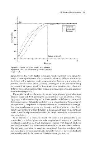
Figure 5.9 Typical variogram models with spherical,
exponential, and Gaussian shapes (sill = 1.0, practical
range = 1.0).

parameters in this work. Spatial correlation, which represents how parameter
values at certain positions can affect or constrain values at a different position, can
be defined with a variogram model. A variogram is a function of a separation lag
distance and it describes spatial variability. A variogram model consists of fitting
an empirical variogram, which is determined from measured data. There are
different shapes of variogram models such as spherical, exponential, and Gaussian
distributions (Figure 5.9).
The spatial dependency of a parameter reduces as the distance between locations
becomes larger and it will converge to an asymptotical value (sill) from a certain
lag (range) as illustrated on Figure 5.9. These models are different in how spatial
dependency reduces. Spherical models decrease in a linear fashion. The decrease of
an exponential is steeper than the spherical model; the local variability is stronger.
Gaussian models decrease gently near the origin and linearly further out so that it
has stronger continuity at short distances. In the uncertainty analysis, the spherical
model is used for all parameters because of the simple linearity and to demonstrate
our methodology.
As an example of a stochastic model, we consider the permeability of an
undisturbed (i.e., before hydraulic stimulation) geothermal reservoir in crystalline
rock based on data from the Urach Spa location (Haenel, 1982). Figure 5.10 shows
one realization result of a permeability distribution for an undisturbed reservoir.
The stochastic generation is based on a conditional Gaussian simulation with
measured data at borehole locations. The parameter values are mapped to the finite
element (FE) mesh for the numerical THM simulation (Section 5.6)