Page 254 - A Practical Guide from Design Planning to Manufacturing

226 Chapter Seven

30

25

Relative frequency 15 Without timing overhead With timing overhead
20

10

5

0
0 5 10 15 20 25 30
Number of pipestages
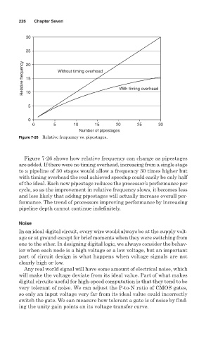
Figure 7-26 Relative frequency vs. pipestages.

Figure 7-26 shows how relative frequency can change as pipestages
are added. If there were no timing overhead, increasing from a single stage
to a pipeline of 30 stages would allow a frequency 30 times higher but
with timing overhead the real achieved speedup could easily be only half
of the ideal. Each new pipestage reduces the processor’s performance per
cycle, so as the improvement in relative frequency slows, it becomes less
and less likely that adding pipestages will actually increase overall per-
formance. The trend of processors improving performance by increasing
pipeline depth cannot continue indefinitely.

Noise
In an ideal digital circuit, every wire would always be at the supply volt-
age or at ground except for brief moments when they were switching from
one to the other. In designing digital logic, we always consider the behav-
ior when each node is a high voltage or a low voltage, but an important
part of circuit design is what happens when voltage signals are not
clearly high or low.
Any real world signal will have some amount of electrical noise, which
will make the voltage deviate from its ideal value. Part of what makes
digital circuits useful for high-speed computation is that they tend to be
very tolerant of noise. We can adjust the P-to-N ratio of CMOS gates,
so only an input voltage very far from its ideal value could incorrectly
switch the gate. We can measure how tolerant a gate is of noise by find-
ing the unity gain points on its voltage transfer curve.