Page 131 - MODELING OF ASPHALT CONCRETE

Complex Modulus Characterization of Asphalt Concr ete 109

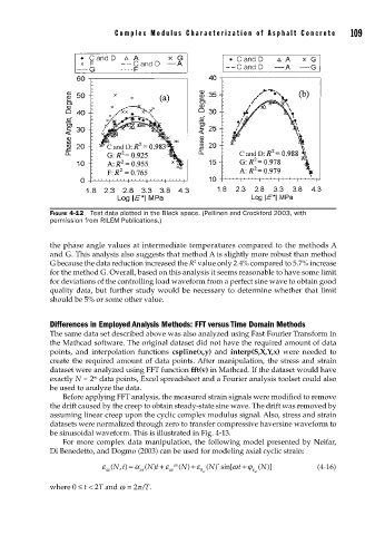
FIGURE 4-12 Test data plotted in the Black space. (Pellinen and Crockford 2003, with
permission from RILEM Publications.)

the phase angle values at intermediate temperatures compared to the methods A
and G. This analysis also suggests that method A is slightly more robust than method
2
G because the data reduction increased the R value only 2.4% compared to 5.7% increase
for the method G. Overall, based on this analysis it seems reasonable to have some limit
for deviations of the controlling load waveform from a perfect sine wave to obtain good
quality data, but further study would be necessary to determine whether that limit
should be 5% or some other value.

Differences in Employed Analysis Methods: FFT versus Time Domain Methods
The same data set described above was also analyzed using Fast Fourier Transform in
the Mathcad software. The original dataset did not have the required amount of data
points, and interpolation functions cspline(x,y) and interp(S,X,Y,x) were needed to
create the required amount of data points. After manipulation, the stress and strain
dataset were analyzed using FFT function fft(v) in Mathcad. If the dataset would have
m
exactly N = 2 data points, Excel spreadsheet and a Fourier analysis toolset could also
be used to analyze the data.
Before applying FFT analysis, the measured strain signals were modified to remove
the drift caused by the creep to obtain steady-state sine wave. The drift was removed by
assuming linear creep upon the cyclic complex modulus signal. Also, stress and strain
datasets were normalized through zero to transfer compressive haversine waveform to
be sinusoidal waveform. This is illustrated in Fig. 4-13.
For more complex data manipulation, the following model presented by Neifar,
Di Benedetto, and Dogmo (2003) can be used for modeling axial cyclic strain:
ε (, = α ( N t + ε av ( N) + ε ( N) sin[ ωt + ϕ ()] (4-16)
*
)
N
Nt)
0
ax
ax
ax
ax ε aax
π
where 0 ≤ t < 2T and ω = 2/T.