Page 132 - MODELING OF ASPHALT CONCRETE

110 Cha pte r F o u r

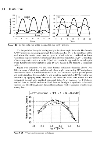
FIGURE 4-13 (a) Raw cyclic data and (b) manipulated data for FFT analysis.

T is the period of the cyclic loading and j is the phase angle of the mix. The formula
ε av () N) is the amplitude of the
N represents the axial permanent deformation and ε (
ax
0 ax
axial sinusoidal strain component at cycle N, which can be considered as linear
viscoelastic response (complex modulus) when creep is eliminated. α ( N) is the slope
ax
of the average deformation at cycles N (and N+1). A similar approach for modeling the
cyclic dynamic modulus signals is used by AAT (2001) in the method G discussed
earlier.
Figure 4-14 compares FFT and time domain techniques discussed above. Two
different ways of obtaining modulus and phase angle values using FFT analysis are
shown in the figure. A method designated as FFT was conducted by manipulating stress
and strain signals as discussed above, and a method designated as FFT-haversine was
conducted by applying fft(v) function to the stress and strain data, which was not
normalized through zero (rectified sinusoidal data). As an example, Fig. 4-13 shows
rectified data on the left and normalized data on the right. A quadratic polynomial
function was fitted through each data set to investigate relative variation of data points
among them.

FIGURE 4-14 FFT versus time domain techniques.