Page 133 - MODELING OF ASPHALT CONCRETE

Complex Modulus Characterization of Asphalt Concr ete 111

The FFT analysis seems to be very close to the method G. However, if the data is
analyzed without normalizing the data through zero (FFT-haversine), the analysis
results were closer to the methods C and D. This indicates that the increased phase
angle values are related to the phase referencing method. The peak picking produces
larger phase angle values than central waveform bracketing due to the skewness of the
stress and strain signals, as was hypothesized in the beginning of the research. However,
the moduli values are not affected in the same extent as Fig. 4-14 shows. This also
explains why the moduli values are not so sensitive for the analysis method compared
to the phase angle values. Therefore, if other than FFT or method G is used for the data
analysis, the phase referencing should be done from the center of the signal to obtain
the phase angle. Based on this analysis, methods A, G, and FFT should be used for
analyzing less perfect sinusoidal cyclic test data. Although this research was done using
dynamic modulus test data, these results can be applied also for shear modulus data or
any sinusoidal cyclic test data.

Mastercurve Development
A full characterization of asphalt mixtures requires one to construct a mastercurve,
which defines the viscoelastic material behavior as a function of both temperature and
loading time.
Time Temperature Superposition Principle
Test data collected at different temperatures can be “shifted” relative to the time of
loading or frequency, so that the various curves can be aligned to form a single
mastercurve. The shift factor a(T) defines the required shift at a given temperature,
that is, a constant by which the time must be divided to get a reduced time for the
mastercurve. In frequency domain, the frequency must be multiplied by shift factor
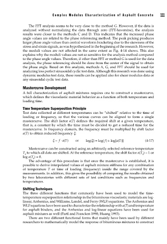
a(T) to obtain reduced frequency x:
⋅
ξ = fa T() or log( ) ξ = log( ) log[ ( )] (4-17)
+
a T
f
Mastercurve can be constructed using an arbitrarily selected reference temperature
T to which all data are shifted. At the reference temperature, the shift factor a(T ) = 1 or
0 0
log a(T ) = 0.
0
The advantage of this procedure is that once the mastercurve is established, it is
possible to derive interpolated values of asphalt mixture stiffness for any combination
of temperature T or time of loading (frequency) inside the range covered by the
measurements. In addition, this gives the possibility of comparing the results obtained
by two laboratories with different sets of test conditions such as frequencies and
temperatures.
Shifting Techniques
The three different functions that commonly have been used to model the time-
temperature superposition relationship in the bituminous viscoelastic materials are log-
linear, Arrhenius, and Williams, Landel, and Ferry (WLF) equations. The Arrhenius and
WLF equations have been used to characterize the relationship with a(T) and temperature
for asphalt binders, and the Arrhenius and log-linear equations have been used for
asphalt mixtures as well (Partl and Francken 1998; Huang 1993).
There are two different functional forms that mainly have been used by different
researchers to mathematically model the response of bituminous mixtures to construct