Page 134 - MODELING OF ASPHALT CONCRETE

112 Cha pte r F o u r

the mastercurve. For time or frequency dependency, the generalized power law has
been used at low to intermediate temperatures when shifting creep or relaxation test
data for asphalt mixtures (Rogue and Buttlar 1992; Christensen 1998). As the higher
temperature data is included, polynomial fitting functions have been used to capture
the form of mastercurve initiated by the material behavior (Francken and Verstraeten
1998). Gordon and Shaw (1994) have used piecewise fitting of polynomial functions
through the test data to construct a mastercurve. Rowe and Sharrock (2000) have
modified this approach by adding the cubic spline method to shift the data to the
reference temperature.

Experimental Shifting and Sigmoidal Fitting Function
A study by Pellinen, Witczak, and Bonaquist (2002) and Pellinen (2001) developed a
method of constructing the full mastercurve using an “experimental” shifting technique
using a sigmoidal fitting function. The experimental shift solves shift factors
simultaneously with the coefficients of the fitting function. In this way the form of the
shift function is not forced to the mastercurve. However, shift factors may absorb some
of the experimental error from the test data.
As mentioned earlier, polynomial fitting functions have been used to shift the
asphalt mix test data using piecewise fitting approach. However, a single polynomial
model cannot be used for fitting the whole mastercurve because the polynomial swing
at low and high temperatures causes irrational modulus value predictions when
extrapolating outside the range of data. To avoid this problem a new functional form,
sigmoidal function Eq. (4-18), was selected to fit the dynamic modulus test data obtained
from temperatures ranging from −18°C to 55°C.
α
log(|E ∗ |) = δ + βγ ξ (4-18)
−
1 + e log( )
∗
where |E | = dynamic modulus
x = reduced frequency
d = minimum modulus value
a = span of modulus values
b, g = shape parameters

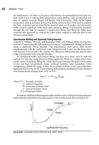
Parameterg influences the steepness of the function (rate of change between minimum
and maximum) and b the horizontal position of the turning point, shown in Fig. 4-15.

FIGURE 4-15 Sigmoidal function (Pellinen et al. 2002, ASCE).