Page 177 - Modern Spatiotemporal Geostatistics

158 Modern Spatiotemporal Geostatistics — Chapter 8

The water-level elevation model

The water-level elevation in the Equus Beds study area was modeled as an
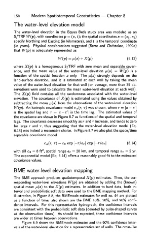
S/TRF W(p), with coordinates p = (s, t); the spatial coordinates s = (s\, s^)
specify Northing and Easting (in kilometers), and t is the temporal coordinate
(in years). Physical considerations suggested (Serre and Christakos, 1999a)
that W(p) is adequately represented as

where X(p) is a homogeneous S/TRF with zero mean and separable covari-
ance, and the mean value of the water-level elevation p,(s) = W(p) is a
function of the spatial location s only. The n(s) strongly depends on the
land-surface elevation, and it is estimated at each well by taking the mean
value of the water-level elevation for that well (on average, more than 35 ob-
servations were used to calculate the mean water-level elevation at each well).
The X(p) field contains all the randomness associated with the water-level
elevation. The covariance of X(p) is estimated using the values obtained by
subtracting the mean /i(s) from the observations of the water-level elevation
W(p). An isotropic covariance model c x(r, r) was chosen, where r = \a - s'\
is the spatial lag and r = \t -1'\ is the time lag. The estimated values of
the covariance are shown in Figure 8.7 as functions of the spatial and temporal
lags. The covariance decreases smoothly as r and r increase, and tends to zero
for large r and r, thus suggesting that the water-level elevation model (Eq.
8.13) was indeed a reasonable choice. In Figure 8.7 we also plot the space/time
separable covariance model

2
with sill CQ = 8 ft , spatial range a r = 20 km, and temporal range a r — 2 yr.
The exponential model (Eq. 8.14) offers a reasonably good fit to the estimated
covariance values.

BME water-level elevation mapping
The BME approach produces spatiotemporal X(p) estimates. Then, the cor-
responding water-level elevations W(p) are obtained by adding the (known)
spatial mean /j,(s) to the X(p) estimates. In addition to hard data, both in-
terval and probabilistic soft data were used by the BME mapping method. For
illustration, in Figure 8.8, the BMEmode estimates for well no. 64 are plotted
as a function of time; also shown are the BME 10%, 50%, and 90% confi-
dence intervals. For this representative hydrograph, the confidence intervals
are consistent with the probabilistic soft data (denoted by pulse-shaped curves
at the observation times). As should be expected, these confidence intervals
are wider at times between observations.
Figure 8.9 shows the BMEmode estimates and the 90% confidence inter-
vals of the water-level elevation for a representative set of wells. The cross-like