Page 251 - Renewable Energy Devices and System with Simulations in MATLAB and ANSYS

238 Renewable Energy Devices and Systems with Simulations in MATLAB and ANSYS ®
®

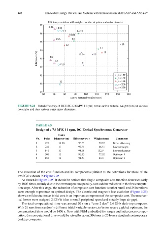
Efficiency variation with weight, number of poles, and outer diameter
97
14.18 14.88
13 14.22
96
12.81
13.5 12
95
12 10
11
94 11
Efficiency (%) 93 13 12 12.14 12

92 12.5 11

91 p=140
p=160
12 p=180
90 p=200
p=220
89
60 70 80 90 100 110 120 130 140
Active material weight (tons)

FIGURE 9.24 Rated efficiency of DCE-SG (7.6 MW, 11 rpm) versus active material weight (tons) at various
pole pairs and thus various outer stator diameters.

TABLE 9.5
Design of a 7.6 MW, 11 rpm, DC-Excited Synchronous Generator

Outer
No. Poles Diameter (m) Efficiency (%) Weight (tons) Comments
1 220 14.18 96.53 70.67 Better efficiency
2 220 13 92.81 66.81 Lowest weight
3 140 10 94.68 132.9 Lowest diameter
4 200 13 96.32 77.02 Optimum 1
5 180 12 94.54 80.0 Optimum 2

The evolution of the cost function and its components (similar to the definitions for those of the
PMSG) is shown in Figure 9.25.
As shown in Figure 9.25, it should be noticed that single-composite cost function decreases early
by 1000 times, mainly due to the overtemperature penalty cost sudden reduction in the first computa-
tion steps. After this stage, the reduction of composite cost function is rather small and 25 iterations
seem enough to produce an optimal design. The electric and magnetic loss evolution (Figure 9.26)
shows a mild reduction as initial cost is an important component of the composite cost. The mechan-
ical losses were assigned 2.92 kW (due to small peripheral speed and notably large air gap).
The total computational time was around 70 s on a “core 2 duo” 2.4 GHz desk-top computer.
With 20 runs from randomly different initial variable vectors, to better secure a global optimum, the
computational time would be 1400 s. Now with FEM embedded for torque and inductances compu-
tation, the computational time would be raised by about 30 times to 25 h on a standard contemporary
desktop computer.