Page 205 - The Geological Interpretation of Well Logs

- THE DIPMETER -

azimuth 360" depth ee dip —. porters . calipers Ww schema E

. 5 - r — -—
. §8., 380 = ==
3 6 ==
“ = |p}
* ¥° aes in Ey
2 = | v
one = __—

° >. . 350 |

Oo Ho ° = [{_ | Lo
e a oo e wu a
eo °| 75 Ss 8B
® * ° °, eo N
° . ° oe *. 5 j}__—_—_——-—__]
eo
. * 490 z ees
— ° u — [_
° é . eo. = wy Y _
+ 42s = A .
74 ol
oO
«f 5 (° ° eee
J_-——-———____]
o 9 . 450 — -c—— eee
=}
586 — | _—--—-—-] -—_—_—_———.
=

hh]
°
go
—
i
=
i
ee
ee
e
>
=
=
75
°
pT
°
=
.
b
>
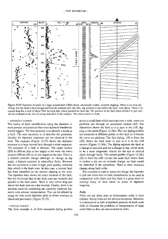
Figure 12.37 Dipmeter example of a sarge normal fault (300m throw, seismically visible, westerly dipping). There is no clear dip
change and the fault is best recognized from the azimuth plot (far left}: dip azimuth is east below the fault, west above. There is no
typica] drag but a zone of about 50m has high dips which parallel the fault dip. The position of the fault plane (if there is just one)
can be proposed at the site of caving indicated on the calipers. The entire section is shale.
— subsurface example across a small fauit which outcrops over a wide, wave-cut
The reality of fault identification using the dipmeter is platform and through an associated vertical cliff. The
more prosaic and practical than most dipmeter handbooks illustration shows the fault as it is seen in the cliff, dip-
would suggest. The first necessity is to identify a break as ping to the north (Figure 12.38a}. The two diplog profiles
a fault. The next necessity is to describe the geometry. are measured at different points on this fault as it crosses
Usually the dipmeter responses are not classical in the the wave-cut platform. The first diplog, 130 m from the
least. The example (Figure 12.37) shows the dipmeter cliff, shows the fault more or less as it is in the cliff
response to a large normal fault through a shale sequence. section (Figure 12.38b). The diplog registers the fault as
The presence of a fault is obvious. The upper section a change in azimuth and not a change in dip, which tends
(300 m-360 m) dips at low angles to the west: the lower to be a more diagnostic feature for the eye in vertical
section (390 m-500 m) at low angles to the east. There is slices through faults. The second profile (Figure 12.38c)
a distinct azimuth change although no change in dip 230 m from the cliff, crosses the same fault where there
angle, a feature common in subsurface faults. Between is neither a dip nor an azimuth change; no fault would
the two sections is a zone of high, poor quality, confused be identified in the subsurface. There is clear character
dips which is the fault zone. In this case, a normal fault change along fault strike.
has been identified on the seismic dipping to the west. This example is used to stress two things: the dipmeter
The dipmeter then shows the exact location of the fault, js just one more tool in fault identification to be used in
that the dominant dips in the fault zone are westerly and conjunction with others and that there is a great need for
parallel to the fault plane. There is very minor drag just outcrop study of fault detail in terms of dipmeter
below the fault seen as a dip reversal. Clearly, there is an response.
absolute need for combining the carefully analysed dip-
meter with seismic interpretation. This can be refined by Folds
using the time scale dipmeter plots in direct overlays as Folds are not often seen in hydrocarbon wells in their
illustrated previously (Figure 12.32). entirety. Slump folds are the obvious exception. However,
it is instructive to look at dipmeter patterns of small scale
— outcrop example folds to illustrate the problems of interpretation of large
The final example is of field measured diplog profiles scale folds as they are encountered in welts.
195