Page 207 - The Geological Interpretation of Well Logs

- THE DIPMETER -

ER
op —= oo ° o Dp =~
4
. 33
ax * ‘ he 4
Ms
‘
b> \\

iz
i
.

14 =
7 i
GG SSA te -—
ye
4
bell

q

‘
we
je
.
: AZ 18 £ €
IN

A. Tight Anticline B. Complex Box Fold
o Dip —a 90° s og Dp — 90°

wu

38
40
scale m
42
aa
C. Anticline (no plunge} D, Plunging at 20°W
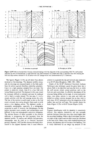
Figure 12.39 Folds on the dipmeter. Outcrop measured diplogs with line diagrams of the corresponding fold. The well symbol
indicates the line of measurement. a) tight anticline, one limb measured; b) comptex box fold; c) anticline with well crossing the
fold axis (dip section, oriented N—S); d} same with a 20° plunge to the west (measurements by G. Cameron).

The figures (Figure 12.39), are all taken from photos solution is to present the dip and azimuth data separately
rendered as line drawings. The dipmeter profiles along- or as SCAT plots (Bengtston, 1980; 1981; 1982).
side the drawings are measured partly in the field, partly Details of the SCAT (Statistica) Curvature Analysis
from the photos and are therefore somewhat schematic. Technique) plot technique cannot be given here, but it
Case A is a tight anticline sampled from one limb. The allows folds to be identified and also the level at which
picture is relativety simple. Case B is a box fold with the well crosses certain unique positions such as the
vertical beds in one limb. The dipmeter in this case would fold axis and axial plane. An effective description of the
be extremely difficult to interpret and may be confused structure being drilled can be made. In some exploration
with a fault or simply missed. The last case, C, is of a areas, even today, seismic is very poor and wells are
simple anticline with the well passing across the crest. drilled on surface outcrop structure just as they were in
The tine of the section is north-south so that as the fold early days. SCAT techniques allow the integration of the
crest is crossed, dips swing abruptly from south to north surface data and the well data. The example shows the
across a low dipping section. The dipmeter profile is fold of figure 12.39c in SCAT format (Figure 12.40).
reasonably interpretable, especially if a sterographic
projection is used. If, however, the fold plunges, the dip Fractures
pattern becomes more complex and interpretation more Fracture identification with the dipmeter is notoriously
difficuit. In this case stereographic analysis is obligatory. difficult. Dip tadpoles themselves will not normally
The obvious feature of these examples is the extreme indicate fractures since they have dips much higher than
difficulty in recognising the fold geometry from the the associated bedding. When a dip is calculated, the Jow-
dipmeter profite. To analyse and identify fold geometry, est angle of dip is taken and two dips cannot be calculated
stereograms may be used as in classical structural at the same leve). Hence, even when marked fractures are
geology (Ramsey, 1967) but this destroys the depth infor- present, the dipmeter dip will be that of the bedding. This
mation in the original dipmeter data, A more effective 197 is nicely illustrated by an image log analysis of the