Page 210 - The Geological Interpretation of Well Logs

- THE GEOLOGICAL INTERPRETATION OF WELL LOGS -

This chapter is written with two objectives in mind: to the gaps between pads remain and they only operate in
describe the way in which the imaging tools work and to water-based muds (Table 13.1). Electric imaging is
show something of the practicalities and results from described in Sections 13.2-13.6.
image interpretation. It is intended for generalists who
Creating an image
will look at logs interpreted by specialists, and not the
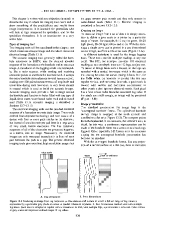
To create an image from a set of data it is simply neces-
specialists themselves. It is an introduction to a very
sary to define a grey scale or a colour by a particular
active field.
range of values. For example, 0-10 may be green, 10-20
Types of imaging tool light green, 20-30 light yellow and so on. With this tech-
Two imaging tools will be considered in this chapter, one nique a single curve can be plotted in a one dimensional
which creates an acoustic image and one which creates an colour image, in effect a colour bar code (Figure 13.1a).
electrical image (Table 13.1). A different technique is used for the image logging
The acoustic imaging tool, generally called the bore- tools. These tools provide multiple readings at any one
hole televiewer or BHTV, uses the detailed acoustic depth. The FMI, for example, provides 192 electrical
response of the formation at the borehole wall to create an readings at any one depth: there are 192 logs, not just one.
image. A transducer on the logging sonde is tured rapid- To create an image from such a dataset, all the logs are
ly, like a radar scanner, while sending and receiving sampled with a vertical increment which is the same as
ultrasonic pulses to and from the borehole wal]. It sweeps the spacing between the curves (being 2.5mm, 0.1", for
the entire borehole circumference-several times a second, the FMI. When the borehole is divided like this into
making over 200 paired measurements of amplitude and regular vertical and horizontal intervals, a patchwork is
trave} time during each revolution. A very dense dataset created with vertical and horizontal co-ordinates: in
is created which is used to build the acoustic images. other words a pixel (picture element) matrix. Each pixel
Acoustic imaging tools provide a full coverage around has a false colour coded from the associated log value. If
the borehole and function in holes filled with any type of the pixels are small enough, an image will be perceived
liquid, fresh water, water-based barite mud and oil-based (Figure 13.18).
mod (Table 13.1). Acoustic imaging is described in
Image presentation
Sections 13.7-13.10.
The standard presentation for image logs is the
The electrical imaging tools use the detailed electrical
‘unwrapped borehole’ format. The cylindrica! borehole
response of a formation to create their image. These tools
surface image is unzipped at the north azimuth and
evolved from dipmeter technology and now consist of a
unrolled to a flat strip (Figure 13.2). The compass points
device with four or more pads similar to the dipmeter,
form the horizontal, X co-ordinates, the vertical Y axis, is
but instead of one electrode per pad there is a large array
depth. In this way, a continuous representation can be
of very small, button electrodes. The fine resistivity
made of the borehole either on a screen or as a hard copy
responses of all of the electrodes are processed together,
log plot. Other, especially 3-D formats exist for on-screen
aS a matrix, into an image. Necessarily, the electrical
display but the unwrapped borehole presentation has
images are only measured immediately in front of each
become the standard.
pad: between the pads is a gap. The present electrical
With the unwrapped borehole format, like any projec-
imaging tools give excellent, high resolution images but
tion of a curved surface on a flat one, there is inevitable
value scale

traces l pixel co-ordinates

depth depth

A. One dimension 8. Two dimensions
Figure 13.1 Producing an image from log responses. A. One dimensional method in which a defined range of log values is
represented by a particular grey shade or colour. A banded column is produced. B. Two dimensional method used with multiple
log traces. Each trace is sampled at regular vertical increments so that, with multiple logs, a pixe] matrix is achieved. False colours
or grey scales stil] represent defined ranges of log values.
200