Page 213 - The Geological Interpretation of Well Logs

- [IMAGE LOGS -

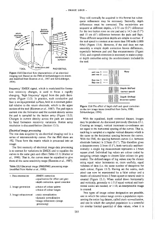
z They will normally be acquired in this format but subse-
°
- quent refinement may be necessary. Secondly, depth
<
2 differences must be corrected. The resistivities are
Cc
o acquired at different depths, a 0.75 cm (0.3") difference
button “
electrade 6 for the two button rows on one pad and a 14.5 cm (5.7")
return current yne
electrade ow and 15 cm (6") difference between the pads and flaps.
{tool} tt
These different acquisition depths are simple to correct if
the tool speed is constant at no more than 550 m/hr (1800
smoothly a simple depth correction leaves differences,
foe insulation fVhr) (Figure 13.6). However, if the tool does not run
flow lines
especially between pad and flap measurements (Figure
PA surfaces er depth correction using the accelerometers included in
13.6), and a speed correction is necessary to make a prop-
equipotential
USL. pad
TOOL PAD DETAIL
pad row 1
Figure 13.5 Electrical flow characteristics of an electrical
pad row 2
imaging tool (based on the FM} of Schlumberger) (re-drawn
and modified from Ekstrom et a/., 1987 and Schlumberger,
flap row 1 ! ,
1994). flap row 2

frequency’ EMEX signal, which is modulated for forma- 4 Depth Shifted
tion resistivity changes, is used to focus a rapidly (correct speed)

changing, ‘high frequency’ signal from the pads them-
Depth Shifted
selves (Figure 13.5). In practice, each conductive pad
{incorrect speed)
face is an equipotential surface, held at a constant poten-
tial relative to the retum electrode, which is the upper
Figure 13.6 The effect of depth shift and speed correction
section of the tool (Ekstrom ef a/., 1987). The pad injects on the raw image traces (modified from Serra, 1989;
current into the formation and the current density across Schlumberger, 1994).
the pad is sampled by the button array (Figure 13.5).
Changes in current density across the pads are caused With the equalised, depth corrected dataset, images
by local formation resistivity variations. Button array may be produced. As discussed previously (Section 13.1,
resolution is discussed below (Section 13.3). Creating an image), vertical increment co-ordinates are
set equal to the horizontal spacing of the curves. That is,
Electrical image processing
each log is sampled at a regular vertical distance which is
The raw data acquired by an electrical imaging tool is a
the same as the horizontal spacing between the curves.
series of microresistivity curves. For the FMI there are
With the FMI, the spacing between curves (i.e. between
192. These form the matrix which is processed into an
electrode buttons) is 2.5mm (0.1"). This therefore gives
image.
a datapoint every 2.5mm (0.1"), both vertically and hori-
The first necessity of electrical image data processing
zontally: a single log measurement represents a 2.5mm
is to correct for variations in EMEX and to equalise the
square pixel. Individual log values are colour coded by
curves to the same gain and offset (Table 13.3) (Harker e¢
assigning certain ranges to chosen false colours (or grey
ai., 1990). That is, the curves must be equalised to give
scales). The defined ranges of log values may be chosen
them all the same sensitivity range (Ekstrom ef ai., 1987).
using equal value increments or, more usefully, equal
Table 13.3 Electrical image (FMS/FMI) processing steps volumes of data (i.e. the same number of datapoints for
(modified from Harker et al., 1990). each colour, Figure 13,7). Having set the scales, each
pixel can now be represented by a false colour and a

1. Data restoration: -EMEX cortection matrix of coloured boxes 2.5mm square at natura] scale is
-equalisation for offset and gain created (Figure 13.1). When scaled down horizontally
—depth correction, speed corection
and vertically, generally to 1:5 if equal vertical and hon-
zontal scales are needed, or 1:10, an interpretable image
2. Image generation —choice of colour palette
—choice of colour ranges is created.
Two types of image colour designation are possible,
3. Image enhancement -static normalisation
one in which the colour range covers a population repre-
—dynamic normalisation
senting the entire log dataset, called static normalisation,
-image refinements (image
and one in which the sampled population is a screenful
processing)
(or similar limited quantity) of data values, when it is

203