Page 330 - Analysis, Synthesis and Design of Chemical Processes, Third Edition

4. Using the random number from Step 3, the value of the parameter is assigned using the
probability distribution (from Step 2) for that parameter.
5. Once values have been assigned to all parameters, these values are used to calculate the
profitability (NPV or other criterion) of the project.
6. Steps 3, 4, and 5 are repeated many times (for example, 1000).
7. A histogram and cumulative probability curve for the profitability criteria calculated from Step 6
are created.
8. The results of Step 7 are used to analyze the profitability of the project.

The algorithm described in this eight-step process is best illustrated by means of an example. However,
before these steps can be completed, it is necessary to review some basic probability theory.

Probability, Probability Distribution, and Cumulative Distribution Functions. A detailed analysis and
description of probability theory are beyond the scope of this book. Instead, some of the basic concepts
and simple distributions are presented. The interested reader is referred to Resnick [5], Valle-Riestra [6],
and Rose [7] for further coverage of this subject.

For any given parameter for which uncertainty exists (and to which some form of distribution will be
assigned), the uncertainty must be described via a probability distribution. The simplest distribution to
use is a uniform distribution, which is illustrated in Figure 10.11.

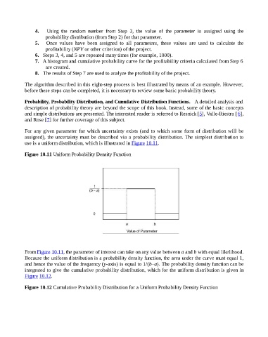
Figure 10.11 Uniform Probability Density Function

From Figure 10.11, the parameter of interest can take on any value between a and b with equal likelihood.
Because the uniform distribution is a probability density function, the area under the curve must equal 1,
and hence the value of the frequency (y-axis) is equal to 1/(b–a). The probability density function can be
integrated to give the cumulative probability distribution, which for the uniform distribution is given in
Figure 10.12.

Figure 10.12 Cumulative Probability Distribution for a Uniform Probability Density Function