Page 69 - Applied Statistics Using SPSS, STATISTICA, MATLAB and R

48 2 Presenting and Summarising the Data

f k = n k/n, where n k is the number of sample values (observations) in bin h k.

The tabular form of the f k is called a frequency table; the graphical form is
known as a histogram. They are representations of estimates of the probability
density function of the associated random variable. Usually the histogram range is
chosen somewhat larger than x h − x l, and adjusted so that convenient limits for the
bins are obtained.
Let d = (x h − x l)/r denote the bin length. Then the probability density estimate
for each of the intervals h k is:

p = d k f
ˆ
k

The areas of the h k intervals are therefore f k and they sum up to 1 as they should.

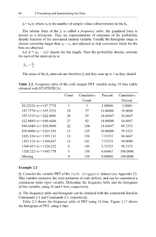
Table 2.2. Frequency table of the cork stopper PRT variable using 10 bins (table
obtained with STATISTICA).

Count Cumulative Percent Cumulative
Count Percent
20.22222<x<=187.7778 3 3 2.00000 2.0000
187.7778<x<=355.3333 24 27 16.00000 18.0000
355.3333<x<=522.8889 28 55 18.66667 36.6667
522.8889<x<=690.4444 27 82 18.00000 54.6667
690.4444<x<=858.0000 22 104 14.66667 69.3333
858.0000<x<=1025.556 15 119 10.00000 79.3333
1025.556<x<=1193.111 11 130 7.33333 86.6667
1193.111<x<=1360.667 11 141 7.33333 94.0000
1360.667<x<=1528.222 8 149 5.33333 99.3333
1528.222<x<=1695.778 1 150 0.66667 100.0000
Missing 0 150 0.00000 100.0000

Example 2.2

Q: Consider the variable PRT of the Cork Stoppers’ dataset (see Appendix E).
This variable measures the total perimeter of cork defects, and can be considered a
continuous (ratio type) variable. Determine the frequency table and the histogram
of this variable, using 10 and 6 bins, respectively.
A: The frequency table and histogram can be obtained with the commands listed in
Commands 2.1 and Commands 2.3, respectively.
Table 2.2 shows the frequency table of PRT using 10 bins. Figure 2.17 shows
the histogram of PRT, using 6 bins.