Page 73 - Applied Statistics Using SPSS, STATISTICA, MATLAB and R

52 2 Presenting and Summarising the Data

represent the probability density estimate for a given bin. We can list de densities
of PRT as follows:

> h$density
[1] 1.333333e-04 1.033333e-03 1.166667e-03
[4] 9.666667e-04 5.666667e-04 4.666667e-04
[7] 4.333333e-04 2.000000e-04 3.333333e-05

Thus, using the formula previously mentioned for the probability density
estimates, we compute the relative frequencies using the bin length (200 in our
case) as follows:

> h$density*200
[1] 0.026666661 0.206666667 0.233333333 0.193333333
[5] 0.113333333 0.093333333 0.086666667 0.040000000
[9] 0.006666667

2.2.3 Multivariate Tables, Scatter Plots and 3D Plots

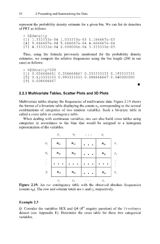
Multivariate tables display the frequencies of multivariate data. Figure 2.19 shows
the format of a bivariate table displaying the counts n ij corresponding to the several
combinations of categories of two random variables. Such a bivariate table is
called a cross table or contingency table.
When dealing with continuous variables, one can also build cross tables using
categories in accordance to the bins that would be assigned to a histogram
representation of the variables.
x x . . . x
1 2 c
y 1 n 11 n 12 . . . n 1c r 1

y 2 n 21 n 22 . . . n 2c r 2

. . . . . . . . . . . . . . . . . .

y r n r1 n r2 . . . n rc r r

c c . . . c
1 2 c
Figure 2.19. An r×c contingency table with the observed absolute frequencies
(counts n ij). The row and column totals are r i and c j, respectively.

Example 2.3
th
Q: Consider the variables SEX and Q4 (4 enquiry question) of the Freshmen
dataset (see Appendix E). Determine the cross table for these two categorical
variables.