Page 70 - Applied Statistics Using SPSS, STATISTICA, MATLAB and R

2.2 Presenting the Data 49

Let X denote the random variable associated to PRT. Then, the histogram of the
frequency values represents an estimate, f ˆ X (x ) , of the unknown probability
density function f X (x ) .
The number of bins to use in a histogram (or in a frequency table) depends on
its goodness of fit to the true density function f X (x ) , in terms of bias and variance.
In order to clarify this issue, let us consider the histograms of PRT using r = 3 and
r = 50 bins as shown in Figure 2.18. Consider in both cases the f ˆ X (x ) estimate
represented by a polygonal line passing through the mid-point values of the
histogram bars. Notice that in the first case (r = 3) the f ˆ X (x ) estimate is quite
smooth and lacks detail, corresponding to a large bias of the expected value
of f ˆ X (x ) – f X (x ) ; i.e., in average terms (for an ensemble of similar histograms
associated to X) the histogram will give a point estimate of the density that can be
quite far from the true density. In the second case (r = 50) the f ˆ X (x ) estimate is
too rough; our polygonal line may pass quite near the true density values, but the
f ˆ X (x ) values vary widely (large variance) around the f X (x ) curve (corresponding
to an average of a large number of such histograms).

50
45

40
35
30
No of obs 25

20
15

10
5
PRT
0
104.000000 606.666667 1109.333333 1612.000000
355.333333 858.000000 1360.666667
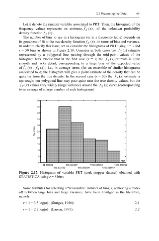
Figure 2.17. Histogram of variable PRT (cork stopper dataset) obtained with
STATISTICA using r = 6 bins.

Some formulas for selecting a “reasonable” number of bins, r, achieving a trade-
off between large bias and large variance, have been divulged in the literature,
namely:
r = 1 + 3.3 log(n) (Sturges, 1926); 2.1

r = 1 + 2.2 log(n) (Larson, 1975). 2.2