Page 322 - DSP Integrated Circuits

7.5 Scheduling Formulations 307

length is 3 bits. The shaded areas indicate execution time for the operations, with
darker shaded areas indicating latency.
If there is a time difference between the
start and the end of a branch, an
implementation would require memory to
be inserted in order to save the output
value until it is needed. The time difference
is referred to as shimming delay. A branch
corresponding to a short difference in time
may be implemented as a cascade of D flip-
flops. For long cascades of D flip-flops, the
Figure 7.28 Direct realization of the
power consumption becomes high, since all
example filter
D flip-flops perform a data transaction in
each clock cycle. Then a cyclic memory may
be more power efficient, since only one input and one output transaction are
required in each clock cycle.
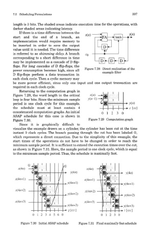
Returning to the computation graph in
Figure 7.29, the word length in the critical
loop is four bits. Since the minimum sample
period is one clock cycle for this example,
the schedule must at least contain 4
concatenated computation graphs. An initial
ASAP schedule for this case is shown in
Figure 7.29 Computation graph
Figure 7.30.
bince it is graphically dimcult to
visualize the example drawn on a cylinder, the cylinder has been cut at the time
instant 0 clock cycles. The branch passing through the cut has been labeled (D,
which represents a direct connection. Due to the simplicity of this example, the
start times of the operations do not have to be changed in order to reach the
minimum sample period. It is sufficient to extend the execution times over the cut,
as shown in Figure 7.31. Here, the sample period is one clock cycle, which is equal
to the minimum sample period. Thus, the schedule is maximally fast.

Figure 7.30 Initial ASAP schedule Figure 7.31 Final maximally fast schedule