Page 572 - Dynamics of Mechanical Systems

0593_C16_fm Page 553 Tuesday, May 7, 2002 7:06 AM

Mechanical Components: Cams 553

Hence, from Eq. (16.8.2) the cam profile radius r(θ) is:

r θ () = r + () (16.9.5)
h θ
0
Using Eq. (16.9.4) produces a profile as in Figure 16.9.4, where a linearly increasing radius
is shown for 90° of the cam angle.

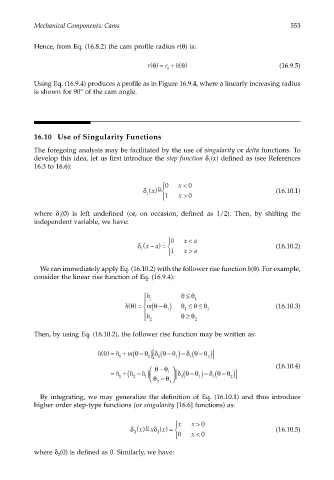
16.10 Use of Singularity Functions
The foregoing analysis may be facilitated by the use of singularity or delta functions. To
develop this idea, let us first introduce the step function δ (x) defined as (see References
1
16.3 to 16.6):

0  x < 0
D
δ x ()=  (16.10.1)
1 x >
 1 0
where δ (0) is left undefined (or, on occasion, defined as 1/2). Then, by shifting the
1
independent variable, we have:

0  x < a
(
−
δ xa) =  (16.10.2)
1 x >
 1 a
We can immediately apply Eq. (16.10.2) with the follower rise function h(θ). For example,
consider the linear rise function of Eq. (16.9.4):

≤
 h 1 θθ 1
(
−
h θ () =  m θθ ) θ ≤≤ 2 (16.10.3)
θ θ

1
1
 θθ
≥
h
 2 2
Then, by using Eq. (16.10.2), the follower rise function may be written as:
m θ θ δ θ θ ) − (
−
h θ () = h + ( − δ θ θ )]
1
1 − ) ( [ 1 1 1 2
−
 θθ  (16.10.4)
δ θ θ )]
= h − )  1 δθ θ ) − ( −
−
h
1 1  θ − θ   ( [ 1 1 1 2
h +( 2
2
1
By integrating, we may generalize the definition of Eq. (16.10.1) and thus introduce
higher order step-type functions (or singularity [16.6] functions) as:
 x x > 0
δ x ()= δ x () =  (16.10.5)
D
x
1
2
 0 x < 0
where δ (0) is defined as 0. Similarly, we have:
2