Page 573 - Dynamics of Mechanical Systems

0593_C16_fm Page 554 Tuesday, May 7, 2002 7:06 AM

554 Dynamics of Mechanical Systems


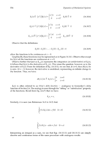
δ x () = ( x 2 2) δ x () =  x 2 2 x > 0 , δ 0 () = 0 (16.10.6)
D
D
1
3
 0 x < 0 3

δ x () = ( x 3 6) δ x () =  x 3 6 x > 0 , δ 0 () = 0 (16.10.7)
D
D
1
4
 0 x < 0 4
n
δ n+1 x () = ( x n) 1  xn! x > 0 , δ n+1 () = 0 (16.10.8)
D
D
δ x () = 
n
0
!
 0 x < 0
Observe that the definitions:
δ 0 () = δ 0 () =…= δ 0 () = δ 0 () = 0 (16.10.9)
2 3 n n + 1
allow the functions to be continuous at x = 0.
Graphically, these functions may be represented as in Figure 16.10.1. Observe that except
for δ (x) all the functions are continuous at x = 0.
1
Observe further that just as δ n+1 (x) represents the integration (or antiderivative) of δ (x),
n
it follows that δ (x) is the derivative of δ n+1 (x). This raises the question, however, as to the
n
derivative of δ (x). From the definition of Eq. (16.10.1), we see that, if x ≠ 0, then dδ (x)/dx
1
1
is zero. At x = 0, however, the derivative is undefined, representing an infinite change in
the function. Thus, we have:

dδ () D δ x () =  0 x ≠ 0 (16.10.10)
x dx =
0
1
 ∞ x = 0
δ (x) is often referred to as Dirac’s delta function — analogous to Kronecker’s delta
0
function of Section 2.6. The analogy is seen through the “sifting” or “substitution” property
of the functions. Recall from Eq. (2.6.7) that we have:
δ v = v (16.10.11)
ij j i

Similarly, it is seen (see References 16.1 to 16.5) that:

b
∫ fx () () f 0 b > ) 0 (16.10.12)
x dx = () (
δ
0
− b
or

b
∫ fx () ( x a dx = () ( b > a) (16.10.13)
− )
δ
f a
0
− b
Interpreting an integral as a sum, we see that Eqs. (16.10.11) and (16.10.11) are simply
discrete and continuous forms of the same procedure with analogous results.