Page 578 - Dynamics of Mechanical Systems

0593_C16_fm Page 559 Tuesday, May 7, 2002 7:06 AM

Mechanical Components: Cams 559

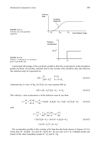
Follower
Rise
Parabolic
Segments

FIGURE 16.11.5
Follower rise with parabolic θ θ θ
segments. 1 m 2 Cam Rotation Angle

a
Follower
Acceleration

2k ω 2

FIGURE 16.11.6
Follower acceleration at transition θ
point to parabolic rise. 1
A principal advantage of the parabolic profile is that the accelerations at the transition
points are finite. To see this, consider that in the vicinity of θ (dwell to rise), the follower
1
rise function may be expressed as:
≤
0 θθ
h θ () =  k θθ ) 2 1 (16.11.2)
(
θ θ
 − 1 θ ≤≤ m
1
Alternatively, in view of Eq. (16.10.2), we may express h(θ) as:
h θ () = ( − 2 δ θ θ ) θ θ (16.11.3)
k θ θ ) (
−
≤
1 1 1 m
The velocity v and acceleration a of the follower near θ are then
1
− )
2
ωθ θ δ
− ) + ωθ θ
v = dh = dh dθ = ω dt = 2 k ( − ) (θ θ k ( − ) (θ θ (16.11.4)
δ
θ
dt d dt dθ 1 1 1 1 0 1
and
2

2
a = dh = d  ω dh dθ = ω 2 dh
θ
θ
dt 2 d  d  dt dθ 2
− ) + 2 ω
− ) (θθ
= k 2 ω δ (θθ k (θ θ δ − ) (16.11.5)
2
2
1 1 1 0 1
− )
k (
+ ωθ θ 1 2 −1 (θ θ 1
− ) δ
2
The acceleration profile in the vicinity of θ then has the form shown in Figure 16.11.6.
1
2
(Note that (θ – θ )δ (θ – θ ) and (θ – θ ) δ (θ – θ ) are zero at θ = θ .) Similar results are
1
1
0
1
1
–1
1
found at the other transition points θ = θ and θ = θ .
m
2