Page 579 - Dynamics of Mechanical Systems

0593_C16_fm Page 560 Tuesday, May 7, 2002 7:06 AM

560 Dynamics of Mechanical Systems

Observe in Figure 16.11.6 that the acceleration is finite in spite of the step jump in its
value. This jump, however, produces an infinite value for the acceleration derivative (often
called the jerk). The jerk (or acceleration derivative) is proportional to the change in inertia
forces. An infinite jerk would then (theoretically) produce an infinite change in the inertia
force which in turn could produce unwanted vibration and wear in the cam–follower pair.
Thus, even though the cam profile is smooth, with no abrupt changes in slope, abrupt
accelerations can still occur for the follower.

16.12 Sinusoidal Rise Function

A second approach to smoothing the motion of the follower is through the use of sinusoidal
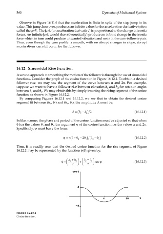
functions. Consider the graph of the cosine function in Figure 16.12.1. To obtain a desired
follower rise, we may use the segment of the curve between π and 2π. For example,
suppose we want to have a follower rise between elevation h and h for rotation angles
1 2
between θ and θ . We may obtain this by simply inserting the rising segment of the cosine
1 2
function as shown in Figure 16.12.2.
By comparing Figures 16.12.1 and 16.12.2, we see that to obtain the desired cosine
segment fit between (h , θ ) and (h , θ ), the amplitude A must be:
1 1 2 2

h − ) 2 (16.12.1)
h
A = ( 2
1
In like manner, the phase and period of the cosine function must be adjusted so that when
θ has the values θ and θ , the argument ψ of the cosine function has the values π and 2π.
1 2
Specifically, ψ must have the form:
ψ = ( + θ − ) (16.12.2)
θ
π θ θ − 2
2 θ ) ( 2 1
1
Then, it is readily seen that the desired cosine function for the rise segment of Figure
16.12.2 may be represented by the function φ(θ) given by:

φ =  h 1 + h 2   +  h 2 − h 1   cos ψ (16.12.3)


2
2

FIGURE 16.12.1
Cosine function.