Page 574 - Dynamics of Mechanical Systems

0593_C16_fm Page 555 Tuesday, May 7, 2002 7:06 AM

Mechanical Components: Cams 555

δ (x)
2
δ (x)
1
1
0 x
0 x
δ (x) δ (x)
3 n
. . .

0 x 0 x
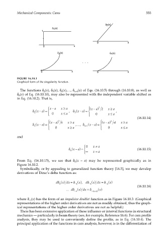
FIGURE 16.10.1
Graphical form of the singularity function.
The functions δ (x), δ (x), δ (x),…, δ n+1 (x) of Eqs. (16.10.5) through (16.10.8), as well as
2
4
3
δ (x) of Eq. (16.10.10), may also be represented with the independent variable shifted as
0
in Eq. (16.10.2). That is,
−
−


(
(
−
−
δ xa) =  xa x ≥ a , δ xa) =  (  xa) 2 2 x ≥ a ,
2
3
 0 x ≤ a  0 x ≤ a

(16.10.14)
−

−

n
3
(
−
−
δ xa) =  (  xa) 6 x ≥ a , …, δ ( xa) =  (  xa) n ! x ≥ a
4 n+ 1
 0 x ≥ a  0 x ≤ a


and

(
−
δ xa) =  0 x ≠ a (16.10.15)
0 ∞ x =
 a
From Eq. (16.10.15), we see that δ (x – a) may be represented graphically as in
0
Figure 16.10.2.
Symbolically, or by appealing to generalized function theory [16.5], we may develop
derivatives of Dirac’s delta function as:
dδ () δ x (), dδ () δ x ()
x dx =
x dx =
0 − 1 − 1 − 2
(16.10.16)
x dx =
… dδ () δ −( n 1) x ()
−
+
n
where δ (x) has the form of an impulsive doublet function as in Figure 16.10.3. (Graphical
–1
representations of the higher order derivatives are not as readily obtained, thus the graph-
ical representations of the higher order derivatives are not as helpful.)
There has been extensive application of these influence or interval functions in structural
mechanics — particularly in beam theory (see, for example, Reference 16.6). For cam profile
analysis, they may be used to conveniently define the profile, as in Eq. (16.10.4). The
principal application of the functions in cam analysis, however, is in the differentiation of