Page 330 - Fundamentals of Gas Shale Reservoirs

310 RESOURCE ESTIMATION FOR SHALE GAS RESERVOIRS

probability distributions. There is no limitation to the becomes significant. A large value indicates that fluids flow
number of parameters that can be varied. The distributions easily between the two porous media, while a small value
are typically normal, uniform, triangular, exponential, or indicates that flow between the media is restricted. No
lognormal. These distributions are sampled for volu- widely available literature reports values of λ and ω for the
metric analysis and flow simulation to determine OGIP, Barnett and Eagle Ford shales. However, the storativity ratio
TRR, and RF. Then, these steps are repeated many times is usually in the range of 0.01–0.1. The interporosity flow
–4
to generate frequency and cumulative density plots for coefficient for gas shales is usually in the range of 10 to
–8
OGIP, TRR, and RF. Finally, economic analysis is run to 10 (Fekete, 2012). These ranges are assumed to be repre-
calculate the production from wells that meet economic sentative of shales due to small pore volume of the fractures,
criteria (IRR >20% before federal income tax, payout <5 and due to the large contrast between the permeabilities
years) over production from all wells according to differ- of the fractures and the matrix. The outer boundary is
ent F&DC. defined as a closed rectangle and the well is centered in
the drainage area. Table 14.7 summarizes the reservoir
model used for shale gas reservoir simulation.
14.3 RESOURCE EVALUATION OF SHALE
GAS PLAYS c t f
c c (14.1)
14.3.1 Reservoir Model t f t m
2
r k
Typical completions for shale gas reservoirs are horizontal mul- 4nn 2) w 2 m (forslabblocks n , 1) (14.2)
(
tistage fractured wells. As more knowledge is gained through L k f
microseismic monitoring of these fracture treatments, it appears
that they are likely creating a network of fractures. Thus, two
permeabilities in gas shales need to be considered: matrix and 14.3.2 Well Spacing Determination
system. System permeability is equivalent to matrix perme- Dong et al. (2013) assumed the width of shale gas reservoir
ability enhanced by the contribution of the fracture network. was 1000 ft. For both sides, the margin from the end of
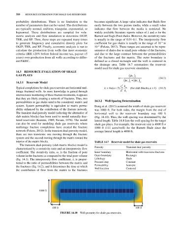
The transient dual‐porosity model (selecting the alternative of horizontal well to the reservoir boundary was 400 ft
slab matrix blocks) has been used to model naturally frac- (Fig. 14.10). Thus, the well spacing was determined by the
tured reservoirs (Kazemi, 1969; Swaan, 1976). The model lateral length. Table 14.8 lists the well spacing for the target
can also be used for modeling shale gas reservoirs where shale gas plays. For example, the reservoir size is 4800 ft ×
multistage fracture completions have created the fracture 1000 ft (111 acres/well) for the Barnett Shale since the
network (Fekete, 2012). In the transient dual‐porosity model, average lateral length is 4000 ft.
there are two transients: one moving through the fracture
system and the second moving through the matrix toward the
interior of the matrix blocks. TAbLE 14.7 Reservoir model for shale gas reservoirs
The transient dual‐porosity (slab matrix blocks) model is
characterized by a storativity ratio and an interporosity flow Porosity Transient dual porosity
coefficient. The storativity ratio, ω, is the fraction of pore Inner boundary Horizontal with transverse fractures
volume in the fractures as compared to the total pore volume Outer boundary Rectangle
(Eq. 14.1). The interporosity flow coefficient, λ, is propor- Lithology Shale
tional to the ratio of permeabilities between the matrix and Pressure step Constant
the fractures (Eq. 14.2), and it determines the time at which Permeability Isotropic
the contribution of flow from the matrix to the fractures Well location Centered

1000 ft

400 ft 400 ft

FIGURE 14.10 Well geometry for shale gas reservoirs.