Page 456 - Industrial Power Engineering and Applications Handbook

14/430 industrial Power Engineering and Applications Handbook
can have a tolerance of up to 25% of the rated frequency short-circuit current, then by using the Simpson formula,
for LT and 10% for HT assemblies. Figure 14.3 illustrates I,, can be calculated by using
a general arrangement for such a test.
.i ,h
I,,, = -[I: +4(1:+ I: +I: +I: +I;)+ 2(I:+ I: + I,' +I:)+ If01
Inference from the oscillogram
r.
This is also known as the asymmetrical breaking current
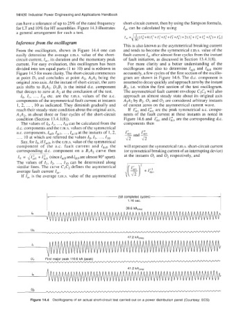
From the oscillogram, shown in Figure 14.4 one can and tends to become the symmetrical r.m.s. value of the
easily determine the average r.m.s. value of the short- fault current I,, aftcr almost four cycles from the instant
circuit current, I,,, its duration and the momentary peak of fault initiation, as discussed in Section 13.4.1(8).
current. For easy evaluation, this oscillogram has been For more clarity and a better understanding of the
divided into ten equal parts (1 to 10) and is redrawn in oscillogram and also to determine Iaco and Ideo more
Figure 14.5 for more clarity. The short-circuit commences accurately, a few cycles of the first section of the oscillo-
at point D1 and concludes at point A2, AIA2 being the gram are shown in Figure 14.6. The d.c. component is
original zero axis. At the instant of short-circuit, the zero assumed to decay quickly and approach zero by the instant
axis shifts to BlA2. DIBl is the initial d.c. component B2, i.e. within the first section of the test oscillogram.
that decays to zero at A, at the conclusion of the test. The asymmetrical fault current envelope C,C4 will also
Z,, 11, ..., Ilo etc. are the r.m.s. values of the a.c. approach an almost steady state about its original axis
components of the asymmetrical fault current at instants AIAz by B2. 0, and O2 are considered arbitrary instants
I, 2, . . . , 10 as indicated. They diminish gradually and of current zeros on the asymmetrical current wave.
reach their steady-state condition about the original axis, If and Z& are the peak symmetrical a.c. compo-
A1A2, in about three or four cycles of the short-circuit nents of the fault current at these instants as noted in
condition (Section 13.4.1(8)). Figure 14.6 and I&, and Z&, are the corresponding d.c.
The values of Z,, I,, . . . , Ilo can be calculated from the components then
d.c. components and the r.m.s. values of the symmctrical
a.c. components, lac,, lac,, ..., Iaclo at the instants of 1, 2,
..., 10 at which are referred the values I,, I,, ..., Ilo.
Say, for Io, if Zaco, is the r.m.s. value of the symmetrical
component of the a.c. fault current and ZdcO the will represent the symmetrical r.m.s. short-circuit current
corresponding d.c. component on a BlA2 curve then (or symmetrical breaking current of an interrupting device)
(since
I, = Jm zac0 and ZdcO are almost 90" apart). at the instants O1 and O2 respectively, and
The values of ZI, I,, ..., I,, can be determined along
similar lines. The curve CI C2 defines the asymmetrical
average fault current ZaV.
If I,, is the average r.m.s. value of the asymmetrical
3

cycles)
completed
(58
sec.
1.16
39.6 kA(,rnS)

UB
Figure 14.4 Oscillograms of an actual short-circuit test carried out on a power distribution panel (Courtesy: ECS)