Page 172 - Separation process principles 2

4.6 Multicomponent Liquid-Liquid Systems 137

4.6 MULTICOMPONENT Most liquid-liquid equilibria are achieved under adia-
LIQUID-LIQUID SYSTEMS batic conditions, thus necessitating consideration of an en-
ergy balance. However, if both feed and solvent enter the
Quarternary and higher multicomponent mixtures are often stage at identical temperatures, the only energy effect is the
encountered in liquid-liquid extraction processes, particu- heat of mixing, which is often sufficiently small that only a
larly when two solvents are used for liquid-liquid extraction. very small temperature change occurs. Accordingly, the cal-
As discussed in Chapter 2, multicomponent liquid-liquid culations are often made isothermally.
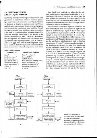
equilibria are very complex and there is no compact graphical The modified Rachford-Rice algorithm is shown in the
way of representing experimental phase equilibria. Accord- flow chart of Figure 4.19. This algorithm is applicable for
ingly, the computation of the equilibrium-phase compositions either an isothermal vapor-liquid (V-L) or liquid-liquid
is best made by a computer-assisted algorithm using activity (L-L) equilibrium-stage calculation when K-values depend
coefficient equations from Chapter 2 that account for the strongly on phase compositions. For the L-L case, the algo-
effect of composition (e.g., NRTL, UNIQUAC, or UNIFAC). rithm assumes that the feed and solvent flow rates and com-
One such algorithm is a modification of the Rachford-Rice positions are fixed. The equilibrium pressure and temperature
algorithm for vapor-liquid equilibrium, given in Tables 4.3 are also specified. An initial estimate is made of the phase
and 4.4. To apply these tables to multicomponent, liquid- compositions, xi') and xiZ), and corresponding estimates of
liquid equilibria, the following symbol transformations are the distribution coefficients are made from liquid-phase
made, where all flow rates and compositions are in moles: activity coefficients, using (2-30) with, for example, the
NRTL or UNIQUAC equations discussed in Chapter 2.
Vapor-Liquid Equilibria
Equation 3 of Table 4.4 is then solved iteratively for
(Tables 4.3,4.4) Liquid-Liquid Equilibria
Q = E/(F + S), from which values of xi2) and x:') are com-
I Feed, F Feed, F, + solvent, S puted from Eqs. (5) and (6), respectively, of Table 4.4. The
j Equilibrium vapor, V Extract, E (L(')) resulting values of x:') and x,(') will not usually sum, respec-
Equilibrium liquid, L Raffinate, R (L(~))
Feed mole fractions, z, Mole fractions of combined F and S tively, to 1 for each liquid phase and are therefore normal-
Vapor mole fractions, y, Extract mole fractions, x,(') ized. The normalized values are obtained from equations
of the form x: = x, / C x,, where xi are the normalized values
Liquid mole fractions, x, Raffinate mole fractions, x,(~)
K-value, K, Distribution coefficient, KD, that force Cxl to equal 1. The normalized values replace
\Ir = V/F q = E/F the values computed from Eqs. (5) and (6). The iterative

Start Start
F, z fixed F, z fixed
P, Tof equilibrium P, T of equilibrium
phases fixed phases fixed

Initial
estimate of x, y
Composition A
&,
Calculate Estimate Calculate Estimate

Iteratively Calculate
New estimate calculatev
I if not direct I
r-l
iteration .I
Calculate x and y
71 Calculate x and y

Figure 4.19 Algorithm for
Compare estimated Normalize x and y.
and calculated Compare estimated isothermal-flash calculation when
and normalized K-values are composition-
converged
converged I exit dependent: (a) separate nested iter-
ations on q and (x, y); (b) simulta-
neous iteration on \I, and (x, y).