Page 41 - Statistics for Environmental Engineers

L1592_frame_C03 Page 32 Tuesday, December 18, 2001 1:41 PM

30

Residual Concentration 10 0 6 4
20

-2 2 0
-4
-6
0 10 20 30
Time (hours)

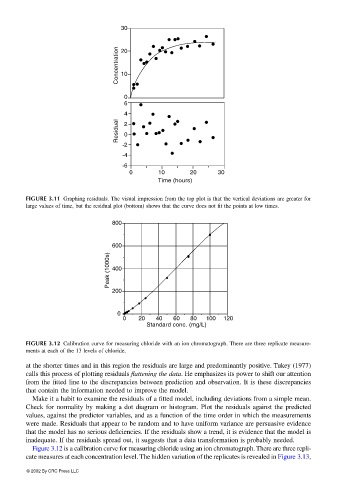
FIGURE 3.11 Graphing residuals. The visual impression from the top plot is that the vertical deviations are greater for
large values of time, but the residual plot (bottom) shows that the curve does not fit the points at low times.

800

600
Peak (1000s) 400

200

0
0 20 40 60 80 100 120
Standard conc. (mg/L)

FIGURE 3.12 Calibration curve for measuring chloride with an ion chromatograph. There are three replicate measure-
ments at each of the 13 levels of chloride.

at the shorter times and in this region the residuals are large and predominantly positive. Tukey (1977)
calls this process of plotting residuals flattening the data. He emphasizes its power to shift our attention
from the fitted line to the discrepancies between prediction and observation. It is these discrepancies
that contain the information needed to improve the model.
Make it a habit to examine the residuals of a fitted model, including deviations from a simple mean.
Check for normality by making a dot diagram or histogram. Plot the residuals against the predicted
values, against the predictor variables, and as a function of the time order in which the measurements
were made. Residuals that appear to be random and to have uniform variance are persuasive evidence
that the model has no serious deficiencies. If the residuals show a trend, it is evidence that the model is
inadequate. If the residuals spread out, it suggests that a data transformation is probably needed.
Figure 3.12 is a calibration curve for measuring chloride using an ion chromatograph. There are three repli-
cate measures at each concentration level. The hidden variation of the replicates is revealed in Figure 3.13,
© 2002 By CRC Press LLC