Page 185 - The Geological Interpretation of Well Logs

- THE DIPMETER -

For example, correlation interval, step distance and Programmes for feature recognition imitate this
search angle must all be defined by the operator and method. Geodip, a Schlumberger programme, mathemat-
therefore can be varied at will. A typical set of parameters ically defines a number of curve features such as large
will be 1.0 m correlation interval, 0.5 m step distance peaks, small peaks, large troughs, etc, and then correlates
(4 correlation, 2’ step are the foot equivalents) and a 50° to similar features in the other curves (Vincent ef al,
search angle. A dip and azimuth value will be given every 1977). Interactive correlation programmes now allow this
50 cm (the step distance) but representing a | m interval. to be done by eye on the screen (Figure 12.7).
This is a relatively coarse set of parameters and is used Feature correlation is made at a defined level, an
for defining ‘structural’ dip (section 12.7): fine features identifiable curve feature is being used. This gives an
will not be measured. The correlation interval may be set, irregular series of dip and azimuth results; where curve
however, at a much smaller value, even down to 10 cm features are good, results are dense: where curves are fea-
(4") on very good quality SHDT logs, which means using tureless there are no results. This clearly has geological
only 40 microresistivity curve sample values (i.e. made implications as will be discussed below (Section 12.7).
every 2.5 mm) for each correlation. An example of a sin- But feature correlation methods are not often used and are
gle set of raw dipmeter data processed with gradually certainly not standard.
varying parameters is shown in Figure 12.18 and dis-
cussed in Section 12.6.
12.4 Processed log presentations
Feature recognition methods Although the ‘tadpole plot’ (see below) is standard for
Microresistivity curve correlation by feature recognition the processed dipmeter log, a number of additional pre-
tries to imitate the way the eye correlates. When correlat- sentations are also available, especially as more dipmeter
ing, the eye picks out a remarkable feature and searches processing software programmes become available.
for a similar feature on the curves to be compared. For Some presentations are general, others unique to one
instance the peak at 2.3 m (Figure 12.7) is picked out service company or one software programme. Some of
easily on all the curves and leads to a visual correlation. these are shown below but the list is not exhaustive.

DEPTH DIP ANGLE AND DIRECTION
_o ee eee GR o MSD results
BOREHOLE 5 190 "Tadpole at 1654m N
RESISTIVITY INCREASES dip = 10°
| azimuth = SE (130°) Ww E
0 10 CALIPERS quality = good
6 16 5
£1-3__ €27-4__ 10/ 20 30 40 50 60 70 80 90
Tee
= 1
od
rT
x
limit of interval “yy Pe oe LU y
a
2 a
for azimuth rose
<--—d
S
diagram a “A wy
(50m intervals) So ? = §

nee SS a

> 2 3s Me

a s GS a

5 ‘ s |
+s
_— 4 $ ASN -
r
are
{1675m) TT
RR
oe STI RIN SS?
aeaye =
FE
4

4
YY
r
SONY
ON
NA
AA
BeOS
ae: at
I

orientation PA “4 |
pad 1 eri aH y iol
_\_-
deviation [Cone 1-3 \ dip grid 0-90° \
grid 0-10° [Cave 2-4
azimuth rose
gamma ray
borehole deviation good quality result (50m interval)
8.5° ESE *reconstituted’
lower quality result
resistivity
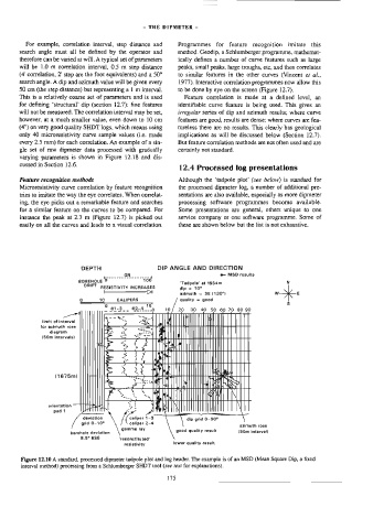
Figure 12.10 A standard, processed dipmeter tadpole plot and log header. The example is of an MSD (Mean Square Dip, a fixed
interval method) processing from a Schlumberger SHDT toot (see text for explanations).
175