Page 186 - The Geological Interpretation of Well Logs

- THE GEOLOGICAL INTERPRETATION OF WELL LOGS -

Simple standard presentation: the ‘tadpole piot’ Acquisition curves
The standard dipmeter presentation is a ‘tadpole plot’ It is a common and useful practice to plot the dipmeter
(Figure 12.10). The basis for the plot is a standard grid microresistivity curves alongside the dipmeter grid and
in which the vertical scale is depth and the horizontal, processed results. The plotted curves are usually edited
variably spaced scale, is dip from 0°-90°. On this grid, and simplified from the raw data but are excellent for
the dip is plotted as a large black dot (the tadpole head) quality control, to indicate textural characteristics and for
whose position has the co-ordinates of depth (from the facies identification (Figures 12.24, 12.29).
vertical scale) and dip (from the horizontal scale). The The acquisition curves are normally plotted on feature
azimuth is then given by a small, straight line (the tadpole recognition processed results logs, such as Geodip and
tail) plotted from the centre of the dot with an orientation Locdip from Schlumberger, so that the level of each
relative to the vertical grid lines which represent true correlation from which a dip is derived may be shown. A
north. On the example log (Figure 12.10), the ‘tadpole’ at quick glance at a Geodip log shows that it has an impor-
1654 m (arrowed) has a dip of 10° with an azimuth to the tant geological content, especially useful in examining
SE of 130°, The tadpole is often varied from the standard sedimentary features (Delhomme and Serra, 1984).
black dot. Square or triangular shapes may be used and
sizes varied. Quality, discussed below (Section 12.5) is Additional plots on standard presentations
frequently indicated by infilled or open shapes, good
— Azimuth rose plot
quality infilled (i.e. solid tadpole ‘head’), poor quality left
Frequently on standard dipmeter tadpole plots, azimuth
open. When colour is used, dip types may be classified or
data are grouped over certain intervals. Typically, on a
a range of qualities indicated by different colours. The
1:500 scale dipmeter log, azimuth data are grouped over
use of the various symbols or colours should be indicated
50 m intervals and plotted as a frequency rose diagram
on each log head.
(Figure 12.10). The azimuth rose is useful in indicating
Accompanying log data unconformities, structural dip direction and faulting.
On standard dipmeter logs processed by service compa- Plotting azimuth roses on pre-determined intervals (i.e.
nies, other information from the tool is plotted besides the each 50 m) however, should be refined by plotting over
dip grid with dip and azimuth values. Typically, this will intervals with meaningful stratigraphic or sedimentary
include the two caliper results, a plot of hole azimuth limits (Figure 12.11). Standard azimuth plots often fail
and drift and a reference log such as a gamma ray or to show important surfaces such as unconformities or
resistivity which allows correlation to the other open hole faults, which have different azimuths, because the pre-
logs. These latter, however, are derived from the dipmeter determined zone straddles the feature (Cameron, 1992),
tool itself, the gamma ray, for example, being from the
gamma ray unit fixed to the dipmeter tool (Section — Dip histogram
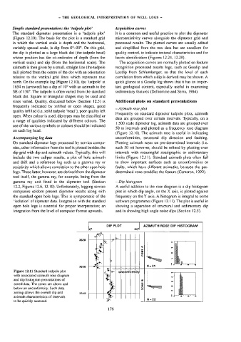
12.2, Figures 12.6, 12.10). Unfortunately, logging service A useful addition to the rose diagram is a dip histogram
companies seldom present dipmeter results along with plot in which dip angle, on the X axis, is plotted against
the standard open hole logs. This is symptomatic of the frequency on the Y axis. A histogram is integral to some
‘isolation’ of dipmeter data. Integration with the standard software programmes (Figure 12.11). The plot is useful in
open hole logs is essential for proper interpretation; an showing a separation of structural and sedimentary dip
integration from the level of computer format upwards. and in showing high angle noise dips (Section 12.5).

DIP PLOT AZIMUTH ROSE DIP HISTOGRAM
oO 90°

lf
oe
3620 .
w
es z
*
§ BL Lb

of
3630
a a
$1 a er et
<
Figure 12.11 Standard tadpole plot Y |@-| unconformity
with associated azimuth rose diagram i
and dip histogram presentations of + a
zoned data. The zones are above and o 2
ad
below an unconformity. Such data iS g
~
. .
r
zoning allows the overall dip and 3640
azimuth characteristics of intervals
to be quickly assessed.
176